Tag: math

  • 5 Simple Steps to Find the Area of Any Figure

    5 Simple Steps to Find the Area of Any Figure

    5 Simple Steps to Find the Area of Any Figure

    $title$

    The world of a determine is a measure of its two-dimensional floor. It may be used to match the sizes of various figures, or to calculate the quantity of fabric wanted to cowl a floor. Discovering the world of a determine is a elementary ability in geometry, and it’s important for a wide range of purposes. On this article, we are going to discover completely different strategies for locating the world of a determine, together with squares, rectangles, triangles, and circles. Our purpose is to empower you with the data and methods vital to find out the world of any determine. As we journey into the realm of geometry, we are going to begin with the only of shapes and regularly progress to extra complicated ones. So, buckle up and prepare to delve into the fascinating world of space measurement!

    One of the primary figures in geometry is a sq.. A sq. is a four-sided determine with 4 equal sides. To search out the world of a sq., we merely have to multiply the size of 1 aspect by itself. For instance, if a sq. has a aspect size of 5 cm, then its space can be 5 cm x 5 cm = 25 cm2. Rectangles are one other frequent determine in geometry. A rectangle is a four-sided determine with two pairs of parallel sides. To search out the world of a rectangle, we multiply the size of the bottom by the peak. For instance, if a rectangle has a base size of 10 cm and a peak of 5 cm, then its space can be 10 cm x 5 cm = 50 cm2.

    Triangles are additionally a typical determine in geometry. A triangle is a three-sided determine. To search out the world of a triangle, we multiply the bottom by the peak after which divide by two. For instance, if a triangle has a base size of 10 cm and a peak of 5 cm, then its space can be 10 cm x 5 cm / 2 = 25 cm2. Circles are a particular kind of determine that’s outlined by its radius. The radius of a circle is the gap from the middle of the circle to any level on the circle. To search out the world of a circle, we use the formulation A = πr2, the place r is the radius of the circle. For instance, if a circle has a radius of 5 cm, then its space can be A = 3.14 x 52 cm2 = 78.5 cm2.

    How To Discover The Space Of A Determine

    The world of a determine is the quantity of area that it takes up. It’s measured in sq. models, corresponding to sq. inches, sq. centimeters, or sq. meters. To search out the world of a determine, you could know its dimensions. For instance, to seek out the world of a rectangle, you could know its size and width. To search out the world of a circle, you could know its radius.

    There are various completely different formulation for locating the world of a determine. The commonest formulation are listed under:

    • Rectangle: Space = size × width
    • Sq.: Space = aspect length²
    • Circle: Space = πr²
    • Triangle: Space = ½ × base × peak
    • Parallelogram: Space = base × peak
    • Trapezoid: Space = ½ × (base₁ + base₂) × peak

    To make use of these formulation, merely plug within the dimensions of the determine into the formulation. For instance, to seek out the world of a rectangle that’s 5 inches lengthy and three inches extensive, you’d use the formulation Space = size × width and plug within the values 5 and three to get an space of 15 sq. inches.

    Individuals Additionally Ask

    How do I discover the world of a determine with no formulation?

    There are just a few alternative ways to seek out the world of a determine with no formulation. A technique is to make use of a grid. To do that, draw a grid over the determine and depend the variety of squares which are contained in the determine. The variety of squares that you simply depend is the world of the determine.

    One other method to discover the world of a determine with no formulation is to make use of a ruler or a measuring tape. To do that, measure the size and width of the determine after which multiply the size by the width to get the world.

    How do I discover the world of an irregular determine?

    To search out the world of an irregular determine, you should utilize a way known as the methodology of decomposition. To do that, divide the irregular determine right into a sequence of smaller, common figures. Then, discover the world of every of the smaller figures and add them collectively to get the world of the irregular determine.

    What’s the distinction between space and perimeter?

    Space and perimeter are two completely different measurements of a determine. Space is the quantity of area {that a} determine takes up, whereas perimeter is the gap across the fringe of a determine. To search out the perimeter of a determine, you could add up the lengths of all the sides of the determine.

  • 5 Simple Steps to Find the Area of Any Figure

    10 Essential Steps to Graphing Polar Equations

    5 Simple Steps to Find the Area of Any Figure

    Delve into the intriguing realm of polar equations, the place curves dance in a symphony of coordinates. In contrast to their Cartesian counterparts, these equations unfold a world of spirals, petals, and different enchanting kinds. To unravel the mysteries of polar graphs, embark on a journey by means of their distinctive visible tapestry.

    The polar coordinate system, with its radial and angular dimensions, serves because the canvas upon which these equations take form. Every level is recognized by its distance from the origin (the radial coordinate) and its angle of inclination from the optimistic x-axis (the angular coordinate). By plotting these coordinates meticulously, the intricate patterns of polar equations emerge.

    As you navigate the world of polar graphs, a kaleidoscope of curves awaits your discovery. Circles, spirals, cardioids, limaçons, and rose curves are only a glimpse of the limitless potentialities. Every equation holds its personal distinctive character, revealing the sweetness and complexity that lies inside mathematical expressions. Embrace the problem of graphing polar equations, and let the visible wonders that unfold ignite your creativeness.

    Changing Polar Equations to Rectangular Equations

    Polar equations describe curves within the polar coordinate system, the place factors are represented by their distance from the origin and the angle they make with the optimistic x-axis. To graph a polar equation, it may be useful to transform it to an oblong equation, which describes a curve within the Cartesian coordinate system, the place factors are represented by their horizontal and vertical coordinates.

    To transform a polar equation to an oblong equation, we use the next trigonometric identities:

    • x = r cos(θ)
    • y = r sin(θ)

    the place r is the space from the origin to the purpose and θ is the angle the purpose makes with the optimistic x-axis.

    To transform a polar equation to an oblong equation, we substitute x and y with the above trigonometric identities and simplify the ensuing equation. For instance, to transform the polar equation r = 2cos(θ) to an oblong equation, we substitute x and y as follows:

    • x = r cos(θ) = 2cos(θ)
    • y = r sin(θ) = 2sin(θ)

    Simplifying the ensuing equation, we get the oblong equation x^2 + y^2 = 4, which is the equation of a circle with radius 2 centered on the origin.

    Plotting Factors within the Polar Coordinate System

    The polar coordinate system is a two-dimensional coordinate system that makes use of a radial distance (r) and an angle (θ) to characterize factors in a aircraft. The radial distance measures the space from the origin to the purpose, and the angle measures the counterclockwise rotation from the optimistic x-axis to the road connecting the origin and the purpose.

    To plot a degree within the polar coordinate system, observe these steps:

    1. Begin on the origin.
    2. Transfer outward alongside the radial line at an angle θ from the optimistic x-axis.
    3. Cease on the level when you may have reached a distance of r from the origin.

    For instance, to plot the purpose (3, π/3), you’ll begin on the origin and transfer outward alongside the road at an angle of π/3 from the optimistic x-axis. You’ll cease at a distance of three models from the origin.

    Radial Distance (r) Angle (θ) Level (r, θ)
    3 π/3 (3, π/3)
    5 π/2 (5, π/2)
    2 3π/4 (2, 3π/4)

    Graphing Polar Equations in Normal Kind (r = f(θ))

    Finding Factors on the Graph

    To graph a polar equation within the type r = f(θ), observe these steps:

    1. Create a desk of values: Select a variety of θ values (angles) and calculate the corresponding r worth for every θ utilizing the equation r = f(θ). This provides you with a set of polar coordinates (r, θ).

    2. Plot the factors: On a polar coordinate aircraft, mark every level (r, θ) in accordance with its radial distance (r) from the pole and its angle (θ) with the polar axis.

    3. Plot Further Factors: To get a extra correct graph, you could need to plot further factors between those you may have already plotted. This may make it easier to determine the form and conduct of the graph.

    Figuring out Symmetries

    Polar equations typically exhibit symmetries primarily based on the values of θ. Listed below are some widespread symmetry properties:

    • Symmetric concerning the x-axis (θ = π/2): If altering θ to -θ doesn’t change the worth of r, the graph is symmetric concerning the x-axis.
    • Symmetric concerning the y-axis (θ = 0 or θ = π): If altering θ to π – θ or -θ doesn’t change the worth of r, the graph is symmetric concerning the y-axis.
    • Symmetric concerning the origin (r = -r): If altering r to -r doesn’t change the worth of θ, the graph is symmetric concerning the origin.
    Symmetry Property Situation
    Symmetric about x-axis r(-θ) = r(θ)
    Symmetric about y-axis r(π-θ) = r(θ) or r(-θ) = r(θ)
    Symmetric about origin r(-r) = r

    Figuring out Symmetries in Polar Graphs

    Inspecting the symmetry of a polar graph can reveal insights into its form and conduct. Listed below are varied symmetry exams to determine various kinds of symmetries:

    Symmetry with respect to the x-axis (θ = π/2):

    Change θ with π – θ within the equation. If the ensuing equation is equal to the unique equation, the graph is symmetric with respect to the x-axis. This symmetry implies that the graph is symmetrical throughout the horizontal line y = 0 within the Cartesian aircraft.

    Symmetry with respect to the y-axis (θ = 0):

    Change θ with -θ within the equation. If the ensuing equation is equal to the unique equation, the graph is symmetric with respect to the y-axis. This symmetry signifies symmetry throughout the vertical line x = 0 within the Cartesian aircraft.

    Symmetry with respect to the road θ = π/4

    Change θ with π/2 – θ within the equation. If the ensuing equation is equal to the unique equation, the graph reveals symmetry with respect to the road θ = π/4. This symmetry implies that the graph is symmetrical throughout the road y = x within the Cartesian aircraft.

    Symmetry Check Equation Transformation Interpretation
    x-axis symmetry θ → π – θ Symmetry throughout the horizontal line y = 0
    y-axis symmetry θ → -θ Symmetry throughout the vertical line x = 0
    θ = π/4 line symmetry θ → π/2 – θ Symmetry throughout the road y = x

    Graphing Polar Equations with Particular Symbologies (e.g., limaçons, cardioids)

    Polar equations typically exhibit distinctive and complex graphical representations. Some particular symbologies characterize particular sorts of polar curves, every with its attribute form.

    Limaçons

    Limaçons are outlined by the equation r = a + bcosθ or r = a + bsinθ, the place a and b are constants. The form of a limaçon is dependent upon the values of a and b, leading to a wide range of kinds, together with the cardioid, debased lemniscate, and witch of Agnesi.

    Cardioid

    A cardioid is a particular kind of limaçon given by the equation r = a(1 + cosθ) or r = a(1 + sinθ), the place a is a continuing. It resembles the form of a coronary heart and is symmetric concerning the polar axis.

    Debased Lemniscate

    The debased lemniscate is one other kind of limaçon outlined by the equation r² = a²cos2θ or r² = a²sin2θ, the place a is a continuing. It has a figure-eight form and is symmetric concerning the x-axis and y-axis.

    Witch of Agnesi

    The witch of Agnesi, outlined by the equation r = a/(1 + cosθ) or r = a/(1 + sinθ), the place a is a continuing, resembles a bell-shaped curve. It’s symmetric concerning the x-axis and has a cusp on the origin.

    Symbology Polar Equation Form
    Limaçon r = a + bcosθ or r = a + bsinθ Varied, relying on a and b
    Cardioid r = a(1 + cosθ) or r = a(1 + sinθ) Coronary heart-shaped
    Debased Lemniscate r² = a²cos2θ or r² = a²sin2θ Determine-eight
    Witch of Agnesi r = a/(1 + cosθ) or r = a/(1 + sinθ) Bell-shaped

    Functions of Polar Graphing (e.g., spirals, roses)

    Spirals

    A spiral is a path that winds round a hard and fast level, getting nearer or farther away because it progresses. In polar coordinates, a spiral will be represented by the equation r = a + bθ, the place a and b are constants. The worth of a determines how shut the spiral begins to the pole, and the worth of b determines how tightly the spiral winds. Optimistic values of b create spirals that wind counterclockwise, whereas adverse values of b create spirals that wind clockwise.

    Roses

    A rose is a curve that consists of a sequence of loops that seem like petals. In polar coordinates, a rose will be represented by the equation r = a sin(nθ), the place n is a continuing. The worth of n determines what number of petals the rose has. For instance, a worth of n = 2 will produce a rose with two petals, whereas a worth of n = 3 will produce a rose with three petals.

    Different Functions

    Polar graphing can be used to characterize a wide range of different shapes, together with cardioids, limaçons, and deltoids. Every kind of form has its personal attribute equation in polar coordinates.

    Form Equation Instance
    Cardioid r = a(1 – cos(θ)) r = 2(1 – cos(θ))
    Limaçon r = a + b cos(θ) r = 2 + 3 cos(θ)
    Deltoid r = a|cos(θ)| r = 3|cos(θ)|

    Remodeling Polar Equations for Graphing

    Changing to Rectangular Kind

    Remodel the polar equation to rectangular type through the use of the next equations:
    x = r cos θ
    y = r sin θ

    Changing to Parametric Equations

    Specific the polar equation as a pair of parametric equations:
    x = r cos θ
    y = r sin θ
    the place θ is the parameter.

    Figuring out Symmetry

    Decide the symmetry of the polar graph primarily based on the next circumstances:
    If r(-θ) = r(θ), the graph is symmetric concerning the polar axis.
    If r(π – θ) = r(θ), the graph is symmetric concerning the horizontal axis (x-axis).
    If r(π + θ) = r(θ), the graph is symmetric concerning the vertical axis (y-axis).

    Discovering Intercepts and Asymptotes

    Discover the θ-intercepts by fixing r = 0.
    Discover the radial asymptotes (if any) by discovering the values of θ for which r approaches infinity.

    Sketching the Graph

    Plot the intercepts and asymptotes (if any).
    Use the symmetry and different traits to sketch the remaining components of the graph.

    Utilizing a Graphing Calculator or Software program

    Enter the polar equation right into a graphing calculator or software program to generate a graph.

    Methodology of Instance: Sketching the Graph of r = 2 + cos θ

    Step 1: Convert to rectangular type:
    x = (2 + cos θ) cos θ
    y = (2 + cos θ) sin θ

    Step 2: Discover symmetry:
    r(-θ) = 2 + cos(-θ) = 2 + cos θ = r(θ), so the graph is symmetric concerning the polar axis.

    Step 3: Discover intercepts:
    r = 0 when θ = π/2 + nπ, the place n is an integer.

    Step 4: Discover asymptotes:
    No radial asymptotes.

    Step 5: Sketch the graph:
    The graph is symmetric concerning the polar axis and has intercepts at (0, π/2 + nπ). It resembles a cardioid.

    Utilizing the Graph to Resolve Equations and Inequalities

    The graph of a polar equation can be utilized to unravel equations and inequalities. To resolve an equation, discover the factors the place the graph crosses the horizontal or vertical strains by means of the origin. The values of the variable corresponding to those factors are the options to the equation.

    To resolve an inequality, discover the areas the place the graph is above or beneath the horizontal or vertical strains by means of the origin. The values of the variable corresponding to those areas are the options to the inequality.

    Fixing Equations

    To resolve an equation of the shape r = a, discover the factors the place the graph of the equation crosses the circle of radius a centered on the origin. The values of the variable corresponding to those factors are the options to the equation.

    To resolve an equation of the shape θ = b, discover the factors the place the graph of the equation intersects the ray with angle b. The values of the variable corresponding to those factors are the options to the equation.

    Fixing Inequalities

    To resolve an inequality of the shape r > a, discover the areas the place the graph of the inequality is exterior of the circle of radius a centered on the origin. The values of the variable corresponding to those areas are the options to the inequality.

    To resolve an inequality of the shape r < a, discover the areas the place the graph of the inequality is inside the circle of radius a centered on the origin. The values of the variable corresponding to those areas are the options to the inequality.

    To resolve an inequality of the shape θ > b, discover the areas the place the graph of the inequality is exterior of the ray with angle b. The values of the variable corresponding to those areas are the options to the inequality.

    To resolve an inequality of the shape θ < b, discover the areas the place the graph of the inequality is inside the ray with angle b. The values of the variable corresponding to those areas are the options to the inequality.

    Instance

    Resolve the equation r = 2.

    The graph of the equation r = 2 is a circle of radius 2 centered on the origin. The options to the equation are the values of the variable akin to the factors the place the graph crosses the circle. These factors are (2, 0), (2, π), (2, 2π), and (2, 3π). Subsequently, the options to the equation r = 2 are θ = 0, θ = π, θ = 2π, and θ = 3π.

    Exploring Conic Sections in Polar Coordinates

    Conic sections are a household of curves that may be generated by the intersection of a aircraft with a cone. In polar coordinates, the equations of conic sections will be simplified to particular kinds, permitting for simpler graphing and evaluation.

    Varieties of Conic Sections

    Conic sections embody: circles, ellipses, parabolas, and hyperbolas. Every kind has a singular equation in polar coordinates.

    Circle

    A circle with radius r centered on the origin has the equation r = r.

    Ellipse

    An ellipse with heart on the origin, semi-major axis a, and semi-minor axis b, has the equation r = a/(1 – e cos θ), the place e is the eccentricity (0 – 1).

    Parabola

    A parabola with focus on the origin and directrix on the polar axis has the equation r = ep/(1 + e cos θ), the place e is the eccentricity (0 – 1) and p is the space from the main target to the directrix.

    Hyperbola

    A hyperbola with heart on the origin, transverse axis alongside the polar axis, and semi-transverse axis a, has the equation r = ae/(1 + e cos θ), the place e is the eccentricity (higher than 1).

    Sort Equation
    Circle r = r
    Ellipse r = a/(1 – e cos θ)
    Parabola r = ep/(1 + e cos θ)
    Hyperbola r = ae/(1 + e cos θ)

    Polar Graphing Methods

    Polar graphing entails plotting factors in a two-dimensional coordinate system utilizing the polar coordinate system. To graph a polar equation, begin by changing it to rectangular type after which find the factors. The equation will be rewritten within the following type:

    x = r cos(theta)

    y = r sin(theta)

    the place ‘r’ represents the space from the origin to the purpose and ‘theta’ represents the angle measured from the optimistic x-axis.

    Superior Polar Graphing Methods (e.g., parametric equations)

    Parametric equations are a flexible device for graphing polar equations. In parametric type, the polar coordinates (r, theta) are expressed as features of a single variable, typically denoted as ‘t’. This enables for the creation of extra advanced and dynamic graphs.

    To graph a polar equation in parametric type, observe these steps:

    1. Rewrite the polar equation in rectangular type:

    x = r cos(theta)

    y = r sin(theta)

    2. Substitute the parametric equations for ‘r’ and ‘theta’:

    x = f(t) * cos(g(t))

    y = f(t) * sin(g(t))

    3. Plot the parametric equations utilizing the values of ‘t’ that correspond to the specified vary of values for ‘theta’.

    Instance: Lissajous Figures

    Lissajous figures are a kind of parametric polar equation that creates intricate and mesmerizing patterns. They’re outlined by the next parametric equations:

    x = A * cos(omega_1 * t)

    y = B * sin(omega_2 * t)

    the place ‘A’ and ‘B’ are the amplitudes and ‘omega_1’ and ‘omega_2’ are the angular frequencies.

    omega_2/omega_1 Form
    1 Ellipse
    2 Determine-eight
    3 Lemniscate
    4 Butterfly

    Learn how to Graph Polar Equations

    Polar equations categorical the connection between a degree and its distance from a hard and fast level (pole) and the angle it makes with a hard and fast line (polar axis). Graphing polar equations entails plotting factors within the polar coordinate aircraft, which is split into quadrants just like the Cartesian coordinate aircraft.

    To graph a polar equation, observe these steps:

    1. Plot the pole on the origin of the polar coordinate aircraft.
    2. Select a beginning angle, sometimes θ = 0 or θ = π/2.
    3. Use the equation to find out the corresponding distance r from the pole for the chosen angle.
    4. Plot the purpose (r, θ) within the acceptable quadrant.
    5. Repeat steps 3 and 4 for extra angles to acquire extra factors.
    6. Join the plotted factors to type the graph of the polar equation.

    Polar equations can characterize varied curves, reminiscent of circles, spirals, roses, and cardioids.

    Individuals Additionally Ask About Learn how to Graph Polar Equations

    How do you discover the symmetry of a polar equation?

    To find out the symmetry of a polar equation, examine if it satisfies the next circumstances:

    • Symmetry concerning the polar axis: Change θ with -θ within the equation. If the ensuing equation is equal to the unique equation, the graph is symmetric concerning the polar axis.
    • Symmetry concerning the horizontal axis: Change r with -r within the equation. If the ensuing equation is equal to the unique equation, the graph is symmetric concerning the horizontal axis (θ = π/2).

    How do you graph a polar equation within the type r = a(θ – b)?

    To graph a polar equation within the type r = a(θ – b), observe these steps:

    1. Plot the pole on the origin.
    2. Begin by plotting the purpose (a, 0) on the polar axis.
    3. Decide the course of the curve primarily based on the signal of “a.” If “a” is optimistic, the curve rotates counterclockwise; if “a” is adverse, it rotates clockwise.
    4. Rotate the purpose (a, 0) by an angle b to acquire the start line of the curve.
    5. Plot further factors utilizing the equation and join them to type the graph.
  • The 2025 SAT Prep Guide: Crack the Exam with Confidence

    The 2025 SAT Prep Guide: Crack the Exam with Confidence

    2025 SAT Prep Guide
    SAT Prep Book 2025

    Are you prepared to beat the SAT in 2025? The last word information to dominating the standardized take a look at is right here! Our complete SAT Prep Ebook 2025 gives an in-depth roadmap to success, empowering you with the data and techniques you should excel.

    Inside this indispensable useful resource, you will discover meticulously crafted apply questions that mirror the precise SAT examination. These questions, meticulously designed by skilled educators, should not merely a set of mock issues; they’re an immersive expertise that replicates the testing setting. By partaking with these challenges, you will acquire familiarity with the query sorts and timing constraints, constructing the arrogance and composure vital for achievement on take a look at day.

    Moreover, our SAT Prep Ebook 2025 goes past mere question-and-answer workouts. It unveils confirmed methods and methods to sort out every part of the examination effortlessly. Complete opinions of Studying, Writing and Language, and Math present an intensive understanding of the content material, whereas skilled suggestions and methods aid you maximize your rating. With this invaluable information in your arsenal, the SAT turns into much less a frightening impediment and extra a chance to showcase your educational prowess.

    Final SAT Prep Information for 2025: Dominating the Studying Part

    1. Demystifying the SAT Studying Check

    The SAT Studying part just isn’t merely a take a look at of your vocabulary or comprehension. It assesses your skill to interact with complicated texts effectively and strategically. Listed here are some essential points to think about:

    • Time Administration: The Studying part includes 52 questions unfold throughout 65 minutes. This interprets to a couple of minute per query, emphasizing the necessity for environment friendly studying and time administration.
    • Complexity of Texts: The passages you will encounter will exhibit a variety of complexity, from simple extracts to dense and multifaceted works. Anticipate to face historic paperwork, scientific articles, persuasive essays, and literary excerpts.
    • Interrogative Types: SAT Studying questions delve into varied points of the textual content and demand completely different interrogative methods. Some questions take a look at literal comprehension, whereas others require you to research the writer’s perspective, infer implied meanings, or establish patterns.
    • Reply Selection Nuances: The reply decisions in SAT Studying questions are sometimes refined and intentionally deceptive. It is important to fastidiously scrutinize every choice earlier than deciding on probably the most acceptable one.

    Desk 1: Sorts of SAT Studying Passages

    Passage Sort Key Options
    Literary Fiction Narrative-driven, vivid language, character improvement
    Nonfiction Prose Factual, informational, or argumentative content material
    Pure Science Scientific theories, experiments, or knowledge interpretation
    Social Science Historic occasions, sociological ideas, or psychological views

    Perfecting the Math Methods for High Scores on the 2025 SAT

    Mastering the Calculator and Non-Calculator Sections

    The SAT Math part consists of two sorts of questions: calculator and non-calculator. For the calculator part, it is important to have a complete understanding of the features and capabilities of your calculator and be proficient in utilizing it for complicated operations. Familiarize your self with the order of operations, grouping symbols, and using the sq. root, absolute worth, and reminiscence features.

    For the non-calculator part, develop sturdy psychological math expertise and estimation methods. Follow fixing issues with no calculator to enhance your quantity sense, approximation talents, and time administration. Make the most of frequent sense and logic to reach at cheap options even when exact calculations should not possible.

    Mastering Ideas and Downside Varieties

    The SAT Math part covers varied mathematical ideas and downside sorts. Grasp the important thing ideas in algebra, geometry, trigonometry, and statistics. Examine the properties of numbers, features, equations, triangles, circles, and likelihood distributions. Perceive the various kinds of questions and the precise formulation or theorems required for every sort.

    Follow fixing all kinds of issues to reinforce your comprehension and problem-solving talents. Make the most of completely different approaches, corresponding to algebraic manipulation, geometric reasoning, and statistical evaluation, to resolve issues successfully.

    Using Follow and Evaluation

    Common apply is essential for SAT Math success. Take timed apply exams to simulate the precise testing circumstances and establish areas for enchancment. Analyze your errors to find out patterns in your errors and develop methods to keep away from them sooner or later.

    Make the most of diagnostic instruments and on-line assets to trace your progress and goal particular areas for enchancment. Search steering from math tutors or academics if wanted to make clear ideas and refine your problem-solving expertise.

    Idea Key Formulation/Theorems
    Algebra Quadratic Equation: x = (-b ± √(b² – 4ac)) / 2a
    Geometry Pythagorean Theorem: a² + b² = c²
    Trigonometry Sine: sin(θ) = reverse/hypotenuse
    Statistics Imply: x̄ = Σx/n

    Excessive-Degree Essay Construction

    The SAT essay evaluates your skill to assemble a well-organized and persuasive argument. Start with a compelling introduction that hooks the reader, presents your thesis assertion, and gives a quick overview of your supporting factors. Every physique paragraph ought to deal with a particular facet of your argument, offering proof and evaluation to help your claims. Conclude your essay with a powerful summation that restates your thesis, summarizes your details, and leaves a long-lasting impression on the reader.

    Crafting a Highly effective Introduction

    An distinctive introduction establishes the aim of your essay and captures the reader’s consideration. Begin with an attention-grabbing hook, corresponding to a compelling anecdote, shocking statistic, or thought-provoking query. Clearly state your thesis assertion, which needs to be a particular, controversial declare that you’ll help all through the essay. Present a quick define of your supporting factors to provide the reader a roadmap of your argument.

    Creating Argumentative Physique Paragraphs

    Every physique paragraph ought to delve into a particular facet of your argument, offering proof and evaluation to help your claims. Start with a subject sentence that states the primary level of the paragraph and connects it to the thesis assertion. Use particular examples, statistics, or credible sources to help your assertions. Interact in essential evaluation, explaining how your proof helps your argument and refuting potential counterarguments. Be sure every physique paragraph is well-developed and transitions easily into the following.

    Physique Paragraph Construction Description
    Matter Sentence States the primary level of the paragraph and connects it to the thesis assertion.
    Proof Particular examples, statistics, or credible sources that help your claims.
    Evaluation Explains how your proof helps your argument and refutes potential counterarguments.
    Transition Connects the paragraph to the following and ensures a clean move of concepts.

    Important Ideas for Tackling SAT Language and Expression

    Concentrate on Sentence Construction and Grammar

    Mastering sentence construction and grammar is essential for understanding the textual content and figuring out errors. Examine grammar guidelines completely, specializing in components of speech, sentence sorts, and customary grammatical errors.

    Improve Vocabulary and Idioms

    Broaden your vocabulary by studying extensively and utilizing flashcards. Concentrate on understanding not solely the definitions of phrases but in addition their shades of which means and the way they’re utilized in context. Be accustomed to frequent idioms and their figurative meanings.

    Follow Studying Comprehension

    Learn quite a lot of texts, together with passages from completely different sources and with completely different types. Be taught to establish the primary concept, supporting particulars, and the writer’s objective. Follow answering comprehension questions that require you to research, interpret, and infer data.

    Grasp Idioms and Figurative Language (300 phrases)

    Idioms and figurative language are integral to SAT Language and Expression. Listed here are particular tricks to improve your understanding and proficiency:

    Determine Frequent Idioms: Familiarize your self with a variety of idioms, learning their literal and figurative meanings. Use context clues to interpret idioms in unfamiliar sentences.

    Perceive Figurative Language: Grasp the various kinds of figurative language, corresponding to metaphors, similes, personification, and hyperbole. Acknowledge the writer’s intent and the aim of utilizing figurative language.

    Analyze Connotation and Denotation: Remember that phrases not solely have their dictionary definitions but in addition connotations (implied meanings). Determine the refined shades of which means conveyed by phrases and the way they affect a sentence’s general tone and message.

    Visualize and Interpret: Figurative language typically depends on imagery and sensory experiences. Follow visualizing the scenes or situations described to reinforce your understanding and interpretation.

    Follow and Repetition: The important thing to mastering idioms and figurative language is apply. Interact in common apply workouts by studying difficult texts and analyzing using figurative units. It’s going to enhance your fluency and confidence in recognizing and decoding these parts successfully.

    Idiom Literal Which means Figurative Which means
    Kick the bucket Die Move away
    Hit the books Examine arduous Consider learning

    Time-Saving Methods for Maximizing SAT Rating Potential

    1. Concentrate on Excessive-Yield Areas

    Prioritize learning materials that seems incessantly on the SAT, corresponding to algebra, geometry, and studying passages based mostly on social research and science. By specializing in these matters, you possibly can maximize your rating with much less effort.

    2. Use Strategic Elimination

    When selecting reply decisions, remove choices which can be clearly incorrect first. This narrows down your decisions and will increase the probability of choosing the right reply.

    3. Make the most of Technique of Elimination

    For tough questions, use strategy of elimination to rule out incorrect solutions. Even for those who aren’t positive of the right reply, this method can enhance your possibilities of selecting accurately.

    4. Take Follow Assessments

    Time your self when taking apply exams to simulate the precise SAT expertise. This helps you establish areas the place you should enhance your pacing.

    5. Grasp Time Administration Methods

    Efficient time administration is essential for maximizing your rating:

    Method Description
    Tempo Your self Distribute time equally amongst sections and questions.
    Skip Troublesome Questions Mark tough questions and return to them later to keep away from losing time.
    Use Highlighting and Word-Taking Mark necessary data in passages and questions to avoid wasting time re-reading.
    Guess Strategically Make educated guesses based mostly on the knowledge it’s a must to keep away from leaving questions clean.

    Unlocking the Secrets and techniques of the New SAT: 2025 Version

    Overview of the New SAT

    The redesigned SAT is designed to be extra simple, clear, and related to college students.

    Key Content material Adjustments

    The Studying and Writing sections now emphasize foundational expertise, whereas the Math part focuses on fewer matters.

    Ideas for Success

    Develop a powerful vocabulary, apply timed writing, and deal with the foundational math ideas.

    The Digital SAT

    The 2025 SAT can be administered digitally, offering college students with a extra accessible and environment friendly testing expertise.

    Adaptive Testing

    The SAT now adjusts the issue of questions based mostly on the coed’s efficiency, offering a extra personalised expertise.

    Scoring the New SAT

    The SAT is scored on a scale of 400 to 1600, with 400 factors in every of the 2 major sections: Proof-Primarily based Studying and Writing, and Math.

    Advantages of the New SAT

    The redesigned SAT gives college students with a extra honest and correct evaluation of their expertise, serving to them make knowledgeable selections about their future.

    Transitioning to the 2025 SAT

    College students ought to begin making ready early and use the official SAT Examine Information and apply exams to familiarize themselves with the brand new format.

    SAT Prep Ebook Suggestions

    Beneath are some extremely advisable SAT prep books for the 2025 version:

    Ebook Title Writer Writer
    SAT Prep Black Ebook Mike Barrett McGraw-Hill
    The Official SAT Examine Information School Board School Board
    Erica Meltzer’s The Important Reader Erica Meltzer Impartial
    Kaplan SAT Premier 2025 Kaplan Check Prep Kaplan
    Princeton Assessment SAT Premium Prep, 2025 Princeton Assessment Princeton Assessment

    The Most Up-to-Date Follow Supplies for the 2025 SAT

    ### 7. Sensible Follow Assessments

    School Board gives 8 official SAT apply exams without spending a dime on its web site. These exams are probably the most genuine apply you will get, as they’re written by the identical individuals who create the precise SAT.

    Advantages of Official Follow Assessments

    * Simulate the true SAT expertise
    * Enable you to establish areas for enchancment
    * Present a benchmark in your progress

    Ideas for Taking Official Follow Assessments

    * Take the exams beneath timed circumstances
    * Assessment your solutions fastidiously after every part
    * Analyze your outcomes to establish your strengths and weaknesses

    Check Sections Time Restrict Scoring
    SAT Follow Check 1 Studying, Writing and Language, Math 3 hours 1600
    SAT Follow Check 2 Studying, Writing and Language, Math 3 hours 1600

    Skilled Steerage for Understanding the SAT Rating Reporting System

    Your Rating Report

    Upon finishing the SAT, you’ll obtain a rating report that features:

    • Your general rating (out of 1600)
    • Your part scores (out of 800): Studying, Writing and Language, and Math
    • Your percentile rank, indicating your efficiency relative to different test-takers
    • Your sub-scores for particular sections (e.g., test-specific evaluation for studying)

    Understanding Your Rating

    The SAT rating vary is from 400 to 1600. Intention for a rating within the seventy fifth percentile or larger to extend your possibilities of admission to your required faculty.

    Sub-Scores for Studying

    The SAT Studying part has three sub-scores:

    • Command of Proof: 17 attainable factors
    • Phrases in Context: 17 attainable factors
    • Evaluation in Historical past/Social Research and in Science: 16 attainable factors

    Command of Proof

    This sub-score assesses your skill to seek out and interpret proof from offered passages. You’ll obtain factors for every right reply you present, as much as a complete of 17 factors.

    The Command of Proof sub-score is additional damaged down into three subcategories:

    • Finding proof: 6 attainable factors
    • Analyzing proof: 6 attainable factors
    • Evaluating proof: 5 attainable factors
    Subcategory Description Doable Factors
    Finding proof Discovering proof that helps the query or assertion 6
    Analyzing proof Understanding the which means of the proof and the way it pertains to the query or assertion 6
    Evaluating proof Figuring out the credibility and relevance of the proof 5

    Important Examine Planners for a Profitable 2025 SAT Preparation

    9. Follow Assessments

    Follow exams are essential for simulating the precise SAT expertise. They permit college students to familiarize themselves with the query format, time constraints, and strain of the examination. Intention to take a number of apply exams all through your preparation and analyze your outcomes fastidiously to establish areas for enchancment.

    Advantages of Follow Assessments: 

    1. Simulate the true SAT
    2. Determine strengths and weaknesses
    3. Monitor progress over time
    4. Handle time successfully
    5. Enhance confidence and scale back take a look at nervousness

    Ideas for Taking Follow Assessments: 

    • Take the take a look at beneath timed circumstances
    • Assessment every query fastidiously
    • Do not skip any sections
    • Guess on any questions you are uncertain about
    • Time your self and attempt to full every part on time

    Advisable Follow Assessments: 

    Title Variety of Assessments Format
    Khan Academy 8 On-line, free
    School Board 10 Official, paid
    Princeton Assessment 5 Ebook or on-line, paid

    High Methods for Overcoming SAT Check Anxiousness and Attaining Optimum Efficiency

    1. Embrace a Development Mindset:

    Consider in your skill to enhance by effort and apply. Keep away from perfectionist tendencies and deal with progress.

    2. Perceive the Check:

    Familiarize your self with the SAT format, query sorts, and time constraints. This information builds confidence and reduces nervousness.

    3. Set Sensible Objectives:

    Intention for a rating that’s difficult however achievable. Breaking down the take a look at into smaller targets makes it much less overwhelming.

    4. Follow Repeatedly:

    Constant apply improves expertise and familiarity. Use timed apply exams to simulate examination circumstances and establish areas for enchancment.

    5. Examine Strategically:

    Use efficient examine methods like spaced repetition, lively recall, and targeted note-taking. Prioritize high-yield matters.

    6. Handle Stress:

    Follow rest methods earlier than and in the course of the examination. Interact in deep respiration, mindfulness, or visualization workouts.

    7. Sleep Adequately:

    Get a full night time’s sleep earlier than the take a look at. Relaxation is important for cognitive operate and decreased nervousness.

    8. Train Repeatedly:

    Bodily exercise reduces stress and improves temper. Interact in moderate-intensity train to advertise rest and increase efficiency.

    9. Eat a Wholesome Breakfast:

    A nutritious breakfast gives power and improves cognitive operate. Keep away from high-sugar or processed meals that may result in crashes.

    10. Optimistic Self-Speak:

    Exchange unfavorable ideas with constructive affirmations. Encourage your self, focus in your strengths, and visualize success.

    SAT Prep Ebook 2025

    The SAT Prep Ebook 2025 is probably the most complete and up-to-date SAT preparation information in the marketplace. It comprises all the pieces you should know to ace the SAT, together with skilled suggestions and techniques, apply exams, and detailed reply explanations. The SAT Prep Ebook 2025 is the one SAT prep e-book you should get the rating you need.

    Listed here are among the options that make the SAT Prep Ebook 2025 the very best SAT prep e-book in the marketplace:

    • Skilled suggestions and techniques: The SAT Prep Ebook 2025 comprises skilled suggestions and techniques from prime SAT tutors. The following pointers and techniques will aid you enhance your rating on each part of the SAT.
    • Follow exams: The SAT Prep Ebook 2025 comprises 8 full-length apply exams. These apply exams are the easiest way to organize for the precise SAT. They are going to assist you become familiar with the format of the take a look at and establish your areas of weak point.
    • Detailed reply explanations: The SAT Prep Ebook 2025 comprises detailed reply explanations for each query on the apply exams. These reply explanations will aid you perceive why you bought every query proper or mistaken. They can even aid you be taught out of your errors and enhance your rating on the precise SAT.

    If you’re severe about getting a excessive rating on the SAT, then you definitely want the SAT Prep Ebook 2025. It’s the most complete and up-to-date SAT preparation information in the marketplace. It comprises all the pieces you should know to ace the SAT, together with skilled suggestions and techniques, apply exams, and detailed reply explanations.

    Individuals Additionally Ask

    What’s the greatest SAT prep e-book 2025?

    One of the best SAT prep e-book 2025 is the SAT Prep Ebook 2025. It comprises all the pieces you should know to ace the SAT, together with skilled suggestions and techniques, apply exams, and detailed reply explanations.

    What’s the most complete SAT prep e-book?

    Probably the most complete SAT prep e-book is the SAT Prep Ebook 2025. It comprises all the pieces you should know to ace the SAT, together with skilled suggestions and techniques, apply exams, and detailed reply explanations.

    What’s the easiest way to organize for the SAT?

    The easiest way to organize for the SAT is to take apply exams. The SAT Prep Ebook 2025 comprises 8 full-length apply exams that can assist you become familiar with the format of the take a look at and establish your areas of weak point.

  • 5 Simple Steps to Find the Area of Any Figure

    6 Easy Steps to Factor a Cubic Expression

    5 Simple Steps to Find the Area of Any Figure

    Featured Picture:

    The world of arithmetic encompasses an unlimited array of ideas and strategies that may appear daunting at first look. One such problem that college students typically face is factoring cubic expressions. These intimidating polynomial expressions of the shape ax³ + bx² + cx + d could evoke a way of trepidation. Nonetheless, with the precise strategy and understanding of basic ideas, factoring cubic expressions can change into a manageable activity. Delve into this complete information and unlock the secrets and techniques to simplifying these complicated algebraic expressions.

    To embark on this factoring journey, allow us to start by inspecting the foundational steps. Recognizing the fixed time period and main coefficient, a and d, is essential. If d isn’t equal to 0, we proceed with the following step. Discovering a pair of integers whose product equals d and sum equals b, the coefficient of x², units the stage for our subsequent transfer. If such a pair exists, we will rewrite the cubic expression as a product of a binomial and a quadratic trinomial.

    Upon acquiring this factorization, additional decomposition of the quadratic trinomial could also be potential. By factoring the trinomial, we will categorical the cubic expression as a product of three linear elements. Nonetheless, if the quadratic trinomial is prime, we can’t issue it additional. Nonetheless, the cubic expression continues to be thought-about factored, albeit in an irreducible type. Understanding these steps and making use of them systematically will empower you to beat the problem of factoring cubic expressions with ease and proficiency.

    How To Issue A Cubic Expression

    Factoring a cubic expression means expressing it as a product of three linear elements. The overall type of a cubic expression is ax³ + bx² + cx + d, the place a, b, c, and d are constants and a isn’t equal to 0.

    To issue a cubic expression, you need to use a wide range of strategies, together with:

    • Factoring by grouping
    • Utilizing the sum or distinction of cubes components
    • Utilizing artificial division
    • Utilizing a graphing calculator

    Upon getting factored the cubic expression, you need to use the zero product property to search out its roots.

    Folks Additionally Ask About How To Issue A Cubic Expression

    How do you issue a trinomial?

    To issue a trinomial, you need to use a wide range of strategies, together with:

    • Factoring by grouping
    • Utilizing the sum or distinction of cubes components
    • Utilizing artificial division
    • Utilizing a graphing calculator

    What’s the distinction between a binomial and a trinomial?

    A binomial is a polynomial with two phrases, whereas a trinomial is a polynomial with three phrases.

    How do you discover the roots of a cubic equation?

    To seek out the roots of a cubic equation, you need to use a wide range of strategies, together with:

    • Factoring the cubic expression
    • Utilizing the quadratic components
    • Utilizing a graphing calculator
  • 5 Simple Steps to Find the Area of Any Figure

    5 Simple Steps to Find Standard Deviation with TI 84

    5 Simple Steps to Find the Area of Any Figure

    Unveiling the secrets and techniques of statistics, this complete information will empower you with a step-by-step method to discovering customary deviation utilizing the versatile TI-84 calculator. Commonplace deviation, a vital parameter in information evaluation, quantifies the unfold or dispersion of knowledge factors round their imply, offering helpful insights into the underlying distribution. By harnessing the facility of the TI-84’s superior statistical capabilities, you’ll achieve a deeper understanding of your information and derive significant conclusions.

    Embark on this statistical journey by first coming into your information into the TI-84. Make use of the “STAT” and “EDIT” menus to meticulously enter the values into record variables (e.g., L1, L2). As soon as your information is securely saved, you’ll be able to seamlessly calculate the usual deviation utilizing the “STAT CALC” menu. Navigate to the “1-Var Stats” possibility and choose the record variable containing your information. With a swift press of the “ENTER” key, the TI-84 will unveil the usual deviation, revealing the extent to which your information factors deviate from their central tendency.

    Moreover, the TI-84 affords further statistical prowess. You’ll be able to delve into the world of speculation testing by using the “2-SampStats” and “2-SampTTest” capabilities. Speculation testing means that you can decide whether or not there’s a statistically vital distinction between two units of knowledge, enabling you to make knowledgeable choices based mostly on stable statistical proof. Whether or not you’re a seasoned statistician or a curious explorer of knowledge evaluation, the TI-84 will information you thru the intricacies of statistical calculations with ease and accuracy.

    Understanding Commonplace Deviation

    Commonplace deviation is a statistical measure that quantifies the quantity of variation or dispersion of a set of knowledge from its imply. It supplies insights into how unfold out or clustered the information factors are across the central tendency. A decrease customary deviation signifies that the information factors are extra carefully clustered across the imply, whereas the next customary deviation signifies higher unfold or dispersion of knowledge factors.

    Calculating Commonplace Deviation

    The method for calculating the usual deviation of a pattern is:
    $$sigma = sqrt{frac{1}{N-1}sum_{i=1}^{N}(x_i – overline{x})^2}$$

    the place:
    – $sigma$ represents the pattern customary deviation
    – $N$ is the pattern measurement
    – $x_i$ are the person information factors within the pattern
    – $overline{x}$ is the pattern imply

    For a inhabitants (your entire set of knowledge, not only a pattern), the method is barely completely different:
    $$sigma = sqrt{frac{1}{N}sum_{i=1}^{N}(x_i – mu)^2}$$

    the place $mu$ represents the inhabitants imply.

    Significance of Commonplace Deviation

    Commonplace deviation performs a vital function in statistical evaluation and inference. It helps in understanding the unfold of knowledge, making predictions, and figuring out the reliability of analysis findings. Additionally it is utilized in speculation testing to evaluate the statistical significance of variations between pattern means. Moreover, customary deviation is a key part in lots of statistical strategies, akin to linear regression and confidence intervals.

    Accessing the TI-84 Calculator

    The TI-84 calculator is a robust graphing calculator that can be utilized to carry out a wide range of mathematical operations, together with discovering the usual deviation of an information set. To entry the TI-84 calculator, you will have to:

    1. Activate the calculator by urgent the ON button.
    2. Press the HOME key to return to the house display.
    3. Press the APPS key to open the Apps menu.
    4. Scroll down and choose the Statistics menu.
    5. Choose the 1-Var Stats possibility.

    Now you can enter your information into the calculator. To do that, press the ENTER key to open the information editor. Enter your information into the L1 column, after which press the ENTER key to maneuver to the following row. Repeat this course of till you’ve entered your whole information.

    Upon getting entered your information, you could find the usual deviation by urgent the STAT key. Scroll down and choose the Calc possibility. Choose the 1-Var Stats possibility, after which press the ENTER key. The calculator will show the usual deviation of your information set within the σx discipline.

    Inputting the Knowledge

    To enter information into the TI-84, observe these steps:

    1. Press the “STAT” button and choose “1: Edit”.
    2. Use the arrow keys to navigate to the primary empty cell within the “L1” column.
    3. Enter the primary information worth utilizing the quantity pad. Urgent “ENTER” after coming into every worth will transfer to the following cell within the “L1” column.
    4. Repeat step 3 for all information values.

    The next information set represents the variety of hours of sleep obtained by a gaggle of scholars:

    L1
    7.5
    6.5
    8.0
    7.0
    6.0

    As soon as the information is entered, you’ll be able to proceed to calculate the usual deviation.

    Discovering the Commonplace Deviation Utilizing STAT

    The TI-84 calculator has a built-in statistical operate that can be utilized to seek out the usual deviation of an information set. To make use of this operate, first enter the information set into the calculator by urgent the STAT button, then deciding on the Edit possibility, after which coming into the information into the record editor. As soon as the information set has been entered, press the 2nd button, then the STAT button, after which choose the Calc possibility. From the Calc menu, choose the 1-Var Stats possibility, after which press the Enter button. The calculator will then show the imply, customary deviation, and different statistical data for the information set.

    The next steps present extra detailed directions on find out how to discover the usual deviation utilizing STAT:

    1. Enter the information set into the calculator by urgent the STAT button, then deciding on the Edit possibility, after which coming into the information into the record editor.
    2. Press the 2nd button, then the STAT button, after which choose the Calc possibility.
    3. From the Calc menu, choose the 1-Var Stats possibility, after which press the Enter button.
    4. The calculator will then show the imply, customary deviation, and different statistical data for the information set.

    Contemplating a selected information set:

    For instance, if the information set is {1, 2, 3, 4, 5}, then the usual deviation is 1.58113883. This may be verified by utilizing the next steps:

    1. Enter the information set into the calculator by urgent the STAT button, then deciding on the Edit possibility, after which coming into the information into the record editor as follows:
    2. L1 1 2 3 4 5
    3. Press the 2nd button, then the STAT button, after which choose the Calc possibility.
    4. From the Calc menu, choose the 1-Var Stats possibility, after which press the Enter button.
    5. The calculator will then show the next statistical data:
    6. n 5
      σx 1.58113883
      σn 1.11803398
      3
      minx 1
      Q1 2
      Med 3
      Q3 4
      maxx 5

    Discovering the Commonplace Deviation Utilizing Lists

    Utilizing lists to calculate customary deviation on a TI-84 calculator is a handy methodology, particularly when working with giant datasets. Comply with these steps to seek out the usual deviation utilizing lists:

    1. Enter the Knowledge into Lists

    Create two lists, one for the information values and one for the frequencies of incidence. For instance, when you’ve got information values 2, 4, 6, and eight, and their respective frequencies are 3, 2, 1, and 4, enter the information into L1 and the frequencies into L2.

    2. Test the Frequency Sum

    Be certain that the sum of frequencies in L2 is the same as the overall variety of information factors. On this case, it must be 10 (3 + 2 + 1 + 4).

    3. Calculate the Imply

    Discover the imply of the information values utilizing the imply operate. For L1, enter imply(L1) and retailer the lead to a variable, akin to X.

    4. Calculate the Variance

    Calculate the variance utilizing the sum operate and the sq. operate. Enter the next into the calculator: sum((L1 - X)^2 * L2). Divide this end result by the variety of information factors minus one (9 on this case). Retailer the lead to a variable, akin to V.

    5. Discovering the Commonplace Deviation

    Lastly, calculate the usual deviation by taking the sq. root of the variance. Enter sqrt(V) and retailer the lead to a variable, akin to S. The usual deviation, represented by S, is the sq. root of the variance.

    6. Show the Outcome

    Show the usual deviation on the display by coming into S.

    Here is a abstract of the steps in desk kind:

    Step Method Description
    1 Enter information into L1, frequencies into L2
    2 Test frequency sum = variety of information factors
    3 imply(L1) Calculate the imply
    4 sum((L1 – X)^2 * L2) / (n – 1) Calculate the variance
    5 sqrt(V) Calculate the usual deviation
    6 Show S Show the usual deviation

    Decoding the Commonplace Deviation

    The usual deviation supplies essential details about the unfold of the information. It measures the variability or dispersion of knowledge factors across the imply. A big customary deviation signifies that the information factors are unfold out over a wider vary, whereas a small customary deviation means that the information factors are clustered extra carefully across the imply.

    The usual deviation is an important parameter in statistics and is utilized in varied purposes, together with:

    • Speculation testing: To find out whether or not a pattern is considerably completely different from a recognized inhabitants.
    • Confidence intervals: To estimate the vary inside which the true inhabitants imply is more likely to fall.
    • Regression evaluation: To evaluate the energy of the connection between variables.

    Relating Commonplace Deviation to Variability

    The usual deviation might be interpreted when it comes to its relationship to variability:

    • About 68% of the information lies inside one customary deviation of the imply. Which means that nearly all of the information factors are inside this vary.
    • Roughly 95% of the information falls inside two customary deviations of the imply. Solely a small proportion of knowledge factors are exterior this vary.
    • Almost 99.7% of the information is captured inside three customary deviations of the imply. This vary encompasses an amazing majority of the information factors.
    Share Commonplace Deviations
    68% 1
    95% 2
    99.7% 3

    Limitations of Utilizing the TI-84

    The TI-84 calculator is a robust device for statistical evaluation, however it does have some limitations.

    Reminiscence limitations

    The TI-84 has a restricted quantity of reminiscence, which may make it troublesome to work with giant datasets. In case your dataset is simply too giant, you could want to separate it into smaller chunks or use a special calculator.

    Precision limitations

    The TI-84 is proscribed to 10-digit precision, which implies that it could not be capable to precisely calculate the usual deviation of very giant or very small datasets. For those who want increased precision, you could want to make use of a special calculator or statistical software program.

    Graphical limitations

    The TI-84’s graphical capabilities are restricted, which may make it troublesome to visualise the distribution of your information. If you could create advanced graphs or histograms, you could want to make use of a special calculator or statistical software program.

    Programming limitations

    The TI-84’s programming capabilities are restricted, which may make it troublesome to automate advanced statistical calculations. If you could carry out advanced calculations or create your individual statistical capabilities, you could want to make use of a special calculator or statistical software program.

    Velocity limitations

    The TI-84 isn’t as quick as another calculators or statistical software program, which may make it troublesome to carry out advanced calculations on giant datasets. If you could carry out calculations shortly, you could want to make use of a special calculator or statistical software program.

    Different limitations

    The TI-84 has plenty of different limitations, together with:

    * It can’t calculate the usual deviation of a inhabitants.
    * It can’t calculate the usual deviation of a weighted dataset.
    * It can’t calculate the usual deviation of a fancy dataset.

    If you could carry out any of those calculations, you will have to make use of a special calculator or statistical software program.

    How one can Discover Commonplace Deviation with a TI-84 Calculator

    **Troubleshooting Frequent Errors**

    Error: “MATH ERROR: INVALID ARGUMENTS”

    This error usually happens when utilizing incorrect syntax or coming into non-numerical values. Be certain that the information is entered as an inventory of numbers or a numerical variable, and that the operate syntax is appropriate (e.g., stdDev(record), stdDev(variable)).

    Error: “DIM MISMATCH”

    This error happens when the variety of information factors within the record or variable doesn’t match the anticipated dimensionality of the operate. Affirm that the operate is being referred to as with the right variety of arguments (e.g., for stdDev, a single record or variable is predicted).

    Error: “LIST NOT DEFINED”

    This error happens when the record or variable getting used has not been outlined or assigned a worth. Be certain that the record or variable is correctly outlined within the calculator’s reminiscence earlier than utilizing it with the stdDev operate.

    Error: “SYNTAX ERROR”

    This error signifies an issue with the syntax of the operate name. Confirm that the operate known as with the right quantity and sort of arguments, and that the parentheses and commas are positioned appropriately.

    Error: “VALUE OUT OF RANGE”

    This error happens when the results of the calculation is simply too giant or too small for the calculator to deal with. Rescale the information or use a special methodology to compute the usual deviation.

    Error Troubleshooting
    “MATH ERROR: INVALID ARGUMENTS” – Test syntax

    – Enter numerical values
    “DIM MISMATCH” – Confirm operate argument depend
    “LIST NOT DEFINED” – Outline record or variable
    “SYNTAX ERROR” – Test operate name syntax

    – Right parentheses and commas
    “VALUE OUT OF RANGE” – Rescale information

    – Use different calculation methodology

    **Step 1: Enter the Knowledge into the Calculator**

    Press the “STAT” button and choose “1:Edit”. Enter your information values into the “L1” record.

    **Step 2: Calculate the Imply**

    Press the “STAT” button once more and choose “CALC” then “1:1-Var Stats”. This can calculate the imply of your information and retailer it within the variable “x̄”.

    **Step 3: Calculate the Variance**

    Press the “STAT” button as soon as extra and choose “CALC” then “1:1-Var Stats”. This time, choose “VARIANCE” to calculate the variance of your information and retailer it within the variable “s²”.

    **Step 4: Calculate the Commonplace Deviation**

    The usual deviation is the sq. root of the variance. To calculate it, press the “x²” button, adopted by the “Ans” button (which accommodates the variance). The end result would be the customary deviation, saved within the “Ans” variable.

    **Step 5: Show the Outcome**

    To show the usual deviation, press the “2nd” button adopted by the “Vars” button and choose “Ans” from the record. The calculator will present the usual deviation on the display.

    **Further Sources for Understanding Commonplace Deviation**

    **What’s Commonplace Deviation?**

    Commonplace deviation measures the unfold or variability of a dataset. It signifies how a lot the person values in a dataset deviate from the imply.

    **Interpretation of Commonplace Deviation**

    A small customary deviation signifies that the information values are clustered carefully across the imply. A big customary deviation signifies that the information values are extra unfold out.

    **Commonplace Deviation Method**

    The method for traditional deviation is: σ = √(Σ(x – μ)² / N)

    The place:

    Image Definition
    σ Commonplace deviation

    x Knowledge worth

    μ Imply

    N Variety of information values

    **Instance Calculation**

    Contemplate the dataset {2, 4, 6, 8, 10}. The imply of this dataset is 6. The variance is 4. The usual deviation is √(4) = 2.

    How one can Discover Commonplace Deviation with TI-84

    The usual deviation is a measure of how unfold out a set of knowledge is. It’s calculated by discovering the sq. root of the variance, which is the typical of the squared variations between every information level and the imply.

    To seek out the usual deviation with a TI-84 calculator, observe these steps:

    1. Enter the information into an inventory. To do that, press the “STAT” button, then choose “1:Edit”. Enter the information into the record, urgent the “ENTER” key after every information level.
    2. Press the “STAT” button once more, then choose “CALC”.
    3. Select the “1-Var Stats” possibility.
    4. The calculator will show the usual deviation, together with different statistics, such because the imply, minimal, and most.

    Individuals Additionally Ask

    What’s the distinction between customary deviation and variance?

    The variance is the typical of the squared variations between every information level and the imply. The usual deviation is the sq. root of the variance.

    How can I take advantage of the usual deviation to make inferences a few inhabitants?

    The usual deviation can be utilized to make inferences a few inhabitants by utilizing the traditional distribution. The conventional distribution is a bell-shaped curve that describes the distribution of many pure phenomena. If the information is generally distributed, then the usual deviation can be utilized to calculate the likelihood of an information level falling inside a sure vary.

    How can I discover the usual deviation of a pattern?

    The usual deviation of a pattern might be discovered utilizing the next method:

    σ = √(Σ(x – μ)² / (n – 1))

    the place:

    • σ is the usual deviation
    • x is every information level
    • μ is the imply
    • n is the variety of information factors

  • 5 Simple Steps to Find the Area of Any Figure

    6 Easy Steps to Multiply and Divide Fractions

    5 Simple Steps to Find the Area of Any Figure

    Within the realm of arithmetic, understanding multiply and divide fractions is a elementary ability that kinds the spine of numerous complicated calculations. These operations empower us to unravel real-world issues, starting from figuring out the realm of an oblong prism to calculating the pace of a transferring object. By mastering the artwork of fraction multiplication and division, we unlock a gateway to a world of mathematical prospects.

    To embark on this mathematical journey, allow us to delve into the world of fractions. A fraction represents part of a complete, expressed as a quotient of two integers. The numerator, the integer above the fraction bar, signifies the variety of elements being thought of, whereas the denominator, the integer beneath the fraction bar, represents the full variety of elements in the entire. Understanding this idea is paramount as we discover the intricacies of fraction multiplication and division.

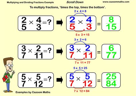
    To multiply fractions, we embark on an easy course of. We merely multiply the numerators of the fractions and the denominators of the fractions, respectively. As an illustration, multiplying 1/2 by 3/4 ends in 1 × 3 / 2 × 4, which simplifies to three/8. This intuitive methodology permits us to mix fractions, representing the product of the elements they characterize. Conversely, division of fractions invitations a slight twist: we invert the second fraction (the divisor) and multiply it by the primary fraction. For example, dividing 1/2 by 3/4 includes inverting 3/4 to 4/3 and multiplying it by 1/2, leading to 1/2 × 4/3, which simplifies to 2/3. This inverse operation permits us to find out what number of occasions one fraction accommodates one other.

    How To Multiply Fractions And Divide

    The Objective of Multiplying Fractions

    Multiplying fractions has numerous sensible purposes in on a regular basis life and throughout completely different fields. Listed here are some key explanation why we use fraction multiplication:

    1. Scaling Portions: Multiplying fractions permits us to scale portions proportionally. As an illustration, if we now have 2/3 of a pizza, and we wish to serve half of it to a buddy, we will calculate the quantity we have to give them by multiplying 2/3 by 1/2, leading to 1/3 of the pizza.

    Unique Quantity Fraction to Scale Consequence
    2/3 pizza 1/2 1/3 pizza

    2. Calculating Charges and Densities: Multiplying fractions is important for figuring out charges and densities. Velocity, for instance, is calculated by multiplying distance by time, which regularly includes multiplying fractions (e.g., miles per hour). Equally, density is calculated by multiplying mass by quantity, which might additionally contain fractions (e.g., grams per cubic centimeter).

    3. Fixing Proportions: Fraction multiplication performs a significant position in fixing proportions. Proportions are equations that state that two ratios are equal. We use fraction multiplication to search out the unknown time period in a proportion. For instance, if we all know that 2/3 is equal to eight/12, we will multiply 2/3 by an element that makes the denominator equal to 12, which on this case is 4.

    2. Step-by-Step Course of

    Multiplying the Numerators and Denominators

    Step one in multiplying fractions is to multiply the numerators of the 2 fractions collectively. The ensuing quantity turns into the numerator of the reply. Equally, multiply the denominators collectively. This outcome turns into the denominator of the reply.

    For instance, let’s multiply 1/2 by 3/4:

    Numerators: 1 * 3 = 3
    Denominators: 2 * 4 = 8

    The product of the numerators is 3, and the product of the denominators is 8. Subsequently, 1/2 * 3/4 = 3/8.

    Simplifying the Product

    After multiplying the numerators and denominators, verify if the outcome might be simplified. Search for widespread elements between the numerator and denominator and divide them out. It will produce the only type of the reply.

    In our instance, 3/8 can’t be simplified additional as a result of there aren’t any widespread elements between 3 and eight. Subsequently, the reply is solely 3/8.

    The Significance of Dividing Fractions

    Dividing fractions is a elementary operation in arithmetic that performs a vital position in numerous real-world purposes. From fixing on a regular basis issues to complicated scientific calculations, dividing fractions is important for understanding and manipulating mathematical ideas. Listed here are a few of the main explanation why dividing fractions is essential:

    Downside-Fixing in Day by day Life

    Dividing fractions is commonly encountered in sensible conditions. As an illustration, if a recipe requires dividing a cup of flour evenly amongst six folks, you’ll want to divide 1/6 of the cup by 6 to find out how a lot every particular person receives. Equally, dividing a pizza into equal slices or apportioning components for a batch of cookies includes utilizing division of fractions.

    Measurement and Proportions

    Dividing fractions is significant in measuring and sustaining proportions. In building, architects and engineers use fractions to characterize measurements, and dividing fractions permits them to calculate ratios for exact proportions. Equally, in science, proportions are sometimes expressed as fractions, and dividing fractions helps decide the focus of gear in options or the ratios of components in chemical reactions.

    Actual-World Calculations

    Division of fractions finds purposes in various fields equivalent to finance, economics, and physics. In finance, calculating rates of interest, forex change charges, or funding returns includes dividing fractions. In economics, dividing fractions helps analyze manufacturing charges, consumption patterns, or price-to-earnings ratios. Physicists use division of fractions when working with power, velocity, or drive, as these portions are sometimes expressed as fractions.

    General, dividing fractions is an important mathematical operation that permits us to unravel issues, make measurements, keep proportions, and carry out complicated calculations in numerous real-world eventualities.

    The Step-by-Step Technique of Dividing Fractions

    Step 1: Decide the Reciprocal of the Second Fraction

    To divide two fractions, you’ll want to multiply the primary fraction by the reciprocal of the second fraction. The reciprocal of a fraction is solely the flipped fraction. For instance, the reciprocal of 1/2 is 2/1.

    Step 2: Multiply the Numerators and Multiply the Denominators

    After you have the reciprocal of the second fraction, you may multiply the numerators and multiply the denominators of the 2 fractions. This provides you with the numerator and denominator of the ensuing fraction.

    Step 3: Simplify the Fraction (Optionally available)

    The ultimate step is to simplify the fraction if attainable. This implies dividing the numerator and denominator by their best widespread issue (GCF). For instance, the fraction 6/8 might be simplified to three/4 by dividing each the numerator and denominator by 2.

    Step 4: Extra Examples

    Let’s observe with a number of examples:

    Instance Step-by-Step Resolution Consequence
    1/2 ÷ 1/4 1/2 x 4/1 = 4/2 = 2 2
    3/5 ÷ 2/3 3/5 x 3/2 = 9/10 9/10
    4/7 ÷ 5/6 4/7 x 6/5 = 24/35 24/35

    Keep in mind, dividing fractions is solely a matter of multiplying by the reciprocal and simplifying the outcome. With just a little observe, you’ll divide fractions with ease!

    Widespread Errors in Multiplying and Dividing Fractions

    Multiplying and dividing fractions might be tough, and it is simple to make errors. Listed here are a few of the most typical errors that college students make:

    1. Not simplifying the fractions first.

    Earlier than you multiply or divide fractions, it is essential to simplify them first. This implies lowering them to their lowest phrases. For instance, 2/4 might be simplified to 1/2, and three/6 might be simplified to 1/2.

    2. Not multiplying the numerators and denominators individually.

    While you multiply fractions, you multiply the numerators collectively and the denominators collectively. For instance, (2/3) * (3/4) = (2 * 3) / (3 * 4) = 6/12.

    3. Not dividing the numerators by the denominators.

    While you divide fractions, you divide the numerator of the primary fraction by the denominator of the second fraction, after which divide the denominator of the primary fraction by the numerator of the second fraction. For instance, (2/3) / (3/4) = (2 * 4) / (3 * 3) = 8/9.

    4. Not multiplying the fractions within the right order.

    While you multiply fractions, it would not matter which order you multiply them in. Nonetheless, if you divide fractions, it does matter. It’s essential to all the time divide the primary fraction by the second fraction.

    5. Not checking your reply.

    As soon as you have multiplied or divided fractions, it is essential to verify your reply to ensure it is right. You are able to do this by multiplying the reply by the second fraction (when you multiplied) or dividing the reply by the second fraction (when you divided). Should you get the unique fraction again, then your reply is right.

    Listed here are some examples of right these errors:

    Error Correction
    2/4 * 3/4 = 6/8 2/4 * 3/4 = (2 * 3) / (4 * 4) = 6/16
    3/4 / 3/4 = 1/1 3/4 / 3/4 = (3 * 4) / (4 * 3) = 1
    4/3 / 3/4 = 4/3 * 4/3 4/3 / 3/4 = (4 * 4) / (3 * 3) = 16/9
    2/3 * 3/4 = 6/12 2/3 * 3/4 = (2 * 3) / (3 * 4) = 6/12 = 1/2

    Functions of Multiplying and Dividing Fractions

    Fractions are a elementary a part of arithmetic and have quite a few purposes in real-world eventualities. Multiplying and dividing fractions is essential in numerous fields, together with:

    Calculating Charges

    Fractions are used to characterize charges, equivalent to pace, density, or stream fee. Multiplying or dividing fractions permits us to calculate the full quantity, distance traveled, or quantity of a substance.

    Scaling Recipes

    When adjusting recipes, we frequently must multiply or divide the ingredient quantities to scale up or down the recipe. By multiplying or dividing the fraction representing the quantity of every ingredient by the specified scale issue, we will guarantee correct proportions.

    Measurement Conversions

    Changing between completely different models of measurement typically includes multiplying or dividing fractions. As an illustration, to transform inches to centimeters, we multiply the variety of inches by the fraction representing the conversion issue (1 inch = 2.54 centimeters).

    Likelihood Calculations

    Fractions are used to characterize the chance of an occasion. Multiplying or dividing fractions permits us to calculate the mixed chance of a number of unbiased occasions.

    Calculating Proportions

    Fractions characterize proportions, and multiplying or dividing them helps us decide the ratio between completely different portions. For instance, in a recipe, the fraction of flour to butter represents the proportion of every ingredient wanted.

    Suggestions for Multiplying Fractions

    When multiplying fractions, multiply the numerators and multiply the denominators:

    Numerators Denominators
    Preliminary Fraction a / b c / d
    Multiplied Fraction a * c / b * d /

    Suggestions for Dividing Fractions

    When dividing fractions, invert the second fraction (divisor) and multiply:

    Numerators Denominators
    Preliminary Fraction a / b c / d
    Inverted Fraction c / d a / b
    Multiplied Fraction a * c / b * d /

    Suggestions for Simplifying Fractions After Multiplication

    After multiplying or dividing fractions, simplify the outcome to its lowest phrases by discovering the best widespread issue (GCF) of the numerator and denominator. There are a number of methods to do that:

    • Prime factorization: Write the numerator and denominator as a product of their prime elements, then cancel out the widespread ones.
    • Factoring utilizing distinction of squares: If the numerator and denominator are excellent squares, use the distinction of squares system (a² – b²) = (a + b)(a – b) to issue out the widespread elements.
    • Use a calculator: If the numbers are giant or the factoring course of is complicated, use a calculator to search out the GCF.

    Instance: Simplify the fraction (8 / 12) * (9 / 15):

    1. Multiply the numerators and denominators: (8 * 9) / (12 * 15) = 72 / 180

    2. Issue the numerator and denominator: 72 = 23 * 32, 180 = 22 * 32 * 5

    3. Cancel out the widespread elements: 22 * 32 = 36, so the simplified fraction is 72 / 180 = 36 / 90 = 2 / 5

    Changing Blended Numbers to Fractions for Division

    When dividing blended numbers, it is necessary to transform them to improper fractions, the place the numerator is bigger than the denominator.

    To do that, multiply the entire quantity by the denominator and add the numerator. The outcome turns into the brand new numerator over the identical denominator.

    For instance, to transform 3 1/2 to an improper fraction, we multiply 3 by 2 (the denominator) and add 1 (the numerator):

    “`
    3 * 2 = 6
    6 + 1 = 7
    “`

    So, 3 1/2 as an improper fraction is 7/2.

    Extra Particulars

    Listed here are some extra particulars to contemplate when changing blended numbers to improper fractions for division:

    • Damaging blended numbers: If the blended quantity is adverse, the numerator of the improper fraction may even be adverse.
    • Improper fractions with completely different denominators: If the blended numbers to be divided have completely different denominators, discover the least widespread a number of (LCM) of the denominators and convert each fractions to improper fractions with the LCM because the widespread denominator.
    • Simplifying the improper fraction: After changing the blended numbers to improper fractions, simplify the ensuing improper fraction, if attainable, by discovering widespread elements and dividing each the numerator and denominator by the widespread issue.
    Blended Quantity Improper Fraction
    2 1/3 7/3
    -4 1/2 -9/2
    5 3/5 28/5

    The Reciprocal Rule for Dividing Fractions

    When dividing fractions, we will use the reciprocal rule. This rule states that the reciprocal of a fraction (a/b) is (b/a). For instance, the reciprocal of 1/2 is 2/1 or just 2.

    To divide fractions utilizing the reciprocal rule, we:

    1. Flip the second fraction (the divisor) to make the reciprocal.
    2. Multiply the numerators and the denominators of the 2 fractions.

    For instance, let’s divide 3/4 by 5/6:

    3/4 ÷ 5/6 = 3/4 × 6/5

    Making use of the multiplication:

    3/4 × 6/5 = (3 × 6) / (4 × 5) = 18/20

    Simplifying, we get:

    18/20 = 9/10

    Subsequently, 3/4 ÷ 5/6 = 9/10.

    Here is a desk summarizing the steps for dividing fractions utilizing the reciprocal rule:

    Step Description
    1 Flip the divisor (second fraction) to make the reciprocal.
    2 Multiply the numerators and denominators of the 2 fractions.
    3 Simplify the outcome if attainable.

    Fraction Division as a Reciprocal Operation

    When dividing fractions, you should use a reciprocal operation. This implies you may flip the fraction you are dividing by the other way up, after which multiply. For instance:

    “`
    3/4 ÷ 1/2 = (3/4) * (2/1) = 6/4 = 3/2
    “`

    The rationale this works is as a result of division is the inverse operation of multiplication. So, when you divide a fraction by one other fraction, you are primarily multiplying the primary fraction by the reciprocal of the second fraction.

    Steps for Dividing Fractions Utilizing the Reciprocal Operation:

    1. Flip the fraction you are dividing by the other way up. That is known as discovering the reciprocal.
    2. Multiply the primary fraction by the reciprocal.
    3. Simplify the ensuing fraction, if attainable.

    Instance:

    “`
    Divide 3/4 by 1/2:

    3/4 ÷ 1/2 = (3/4) * (2/1) = 6/4 = 3/2
    “`

    Desk:

    Fraction Reciprocal
    3/4 4/3
    1/2 2/1

    Find out how to Multiply and Divide Fractions

    Multiplying fractions is straightforward! Simply multiply the numerators (the highest numbers) and the denominators (the underside numbers) of the fractions.

    For instance:

    To multiply 1/2 by 3/4, we multiply 1 by 3 and a couple of by 4, which supplies us 3/8.

    Dividing fractions can also be simple. To divide a fraction, we flip the second fraction (the divisor) and multiply. That’s, we multiply the numerator of the primary fraction by the denominator of the second fraction, and the denominator of the primary fraction by the numerator of the second fraction.

    For instance:

    To divide 1/2 by 3/4, we flip 3/4 and multiply, which supplies us 4/6, which simplifies to 2/3.

    Folks Additionally Ask

    Can we add fractions with completely different denominators?

    Sure, we will add fractions with completely different denominators by first discovering the least widespread a number of (LCM) of the denominators. The LCM is the smallest quantity that’s divisible by all of the denominators.

    For instance:

    So as to add 1/2 and 1/3, we first discover the LCM of two and three, which is 6. Then, we rewrite the fractions with the LCM because the denominator:

    1/2 = 3/6

    1/3 = 2/6

    Now we will add the fractions:

    3/6 + 2/6 = 5/6

  • 5 Simple Steps to Find the Area of Any Figure

    6 Easy Steps: How to Calculate Standard Deviation on TI-84

    5 Simple Steps to Find the Area of Any Figure
    $title$

    When evaluating giant knowledge units, commonplace deviation is a helpful statistical measure of how unfold out the information is. A low commonplace deviation signifies that the information is clustered intently across the imply, whereas a excessive commonplace deviation signifies that the information is extra unfold out. Understanding learn how to calculate commonplace deviation on a TI-84 graphing calculator could be important for knowledge evaluation and interpretation.

    The TI-84 graphing calculator affords a simple methodology for calculating commonplace deviation. First, enter the information into a listing. Press the “STAT” button, choose “EDIT,” and select a listing (L1, L2, and so on.) to enter the information values. As soon as the information is entered, press the “STAT” button once more, choose “CALC,” after which select “1-Var Stats.” This may show numerous statistical calculations, together with the usual deviation (σx). If you must calculate the pattern commonplace deviation (s), press “2nd” after which “STAT” to entry the pattern statistics menu and choose “1-Var Stats.” Bear in mind to regulate the calculation kind accordingly primarily based on whether or not you are working with a inhabitants or a pattern.

    After getting calculated the usual deviation, you possibly can interpret it within the context of your knowledge. A low commonplace deviation means that the information factors are comparatively near the imply, whereas a excessive commonplace deviation signifies that the information factors are extra unfold out. This data could be helpful for making inferences concerning the underlying distribution of the information and drawing significant conclusions out of your evaluation.

    Understanding Customary Deviation

    Customary deviation is a measure of how a lot the information is unfold out. It’s calculated by discovering the sq. root of the variance. Variance is calculated by discovering the typical squared distance between every knowledge level and the imply of the information. The usual deviation is expressed in the identical models as the information.

    As an illustration, if the information is measured in inches, the usual deviation can be in inches. A low commonplace deviation signifies that the information is clustered across the imply, whereas a excessive commonplace deviation signifies that the information is unfold out.

    Customary deviation is a helpful measure for evaluating completely different datasets. For instance, if two datasets have the identical imply, however one dataset has a better commonplace deviation, it signifies that the information in that dataset is extra unfold out.

    Desk: Examples of Customary Deviation

    Dataset Imply Customary Deviation
    Top of scholars in a category 68 inches 4 inches
    Scores on a check 75% 10%
    Weights of new child infants 7 kilos 2 kilos

    Utilizing the TI-84 Calculator

    The TI-84 calculator is a strong statistical instrument that can be utilized to calculate quite a lot of statistical measures, together with commonplace deviation. To calculate the usual deviation of a knowledge set utilizing the TI-84, observe these steps:

    1. Enter the information set into the calculator utilizing the LIST menu.
    2. Calculate the pattern commonplace deviation utilizing the 2nd VARS STAT menu, choosing choice 1 (stdDev).
    3. The pattern commonplace deviation can be displayed on the display screen.

    Clarification of Step 2: Calculating Pattern Customary Deviation

    The TI-84 can calculate each the pattern commonplace deviation (s) and the inhabitants commonplace deviation (σ). The pattern commonplace deviation is the measure of dispersion that’s sometimes used when solely a pattern of knowledge is out there, whereas the inhabitants commonplace deviation is used when your entire inhabitants knowledge is out there. To calculate the pattern commonplace deviation utilizing the TI-84, choose choice 1 (stdDev) from the 2nd VARS STAT menu.

    After choosing choice 1, the calculator will immediate you to enter the record title of the information set. Enter the title of the record the place you could have saved your knowledge, and press ENTER. The calculator will then show the pattern commonplace deviation on the display screen.

    Here’s a desk summarizing the steps to calculate commonplace deviation utilizing the TI-84 calculator:

    Step Description
    1 Enter the information set into the calculator utilizing the LIST menu.
    2 Calculate the pattern commonplace deviation utilizing the 2nd VARS STAT menu, choosing choice 1 (stdDev).
    3 The pattern commonplace deviation can be displayed on the display screen.

    Step-by-Step Directions

    Collect Your Information

    Enter your knowledge into the TI-84 calculator. Press the STAT button, choose “Edit” and enter the information factors into L1 or another accessible record. Be certain that your knowledge is organized and correct.

    Calculate the Imply

    Press the STAT button once more and choose “Calc” from the menu. Scroll all the way down to “1-Var Stats” and press enter. Choose the record containing your knowledge (e.g., L1) and press enter. The calculator will show the imply (common) of the information set. Be aware down this worth as will probably be wanted later.

    Calculate the Variance

    Return to the “Calc” menu and choose “2-Var Stats.” This time, choose “Record” from the primary immediate and enter the record containing your knowledge (e.g., L1) as “Xlist.” Go away the “Ylist” area clean and press enter. The calculator will show the sum of squares (Σx²), the imply (µ), and the variance (s²). The variance represents the typical of the squared variations between every knowledge level and the imply.

    Detailed Clarification of Variance Calculation:

    Variance is a measure of how unfold out the information is from the imply. A better variance signifies that the information factors are extra dispersed, whereas a decrease variance signifies that they’re extra clustered across the imply.

    To calculate the variance utilizing the TI-84, observe these steps:

    1. Press the STAT button.
    2. Choose “Calc” from the menu.
    3. Scroll all the way down to “2-Var Stats.”
    4. Choose “Record” from the primary immediate and enter the record containing your knowledge (e.g., L1) as “Xlist.”
    5. Go away the “Ylist” area clean and press enter.
    6. The calculator will show the sum of squares (Σx²), the imply (µ), and the variance (s²).

      The variance is calculated utilizing the next method:
      “`
      s² = Σx² / (n-1)
      “`
      the place:
      – s² is the variance
      – Σx² is the sum of squares
      – n is the variety of knowledge factors
      – µ is the imply

      Getting into Information into the Calculator

      To calculate the usual deviation on a TI-84 calculator, you will need to first enter the information into the calculator. There are two methods to do that:

      1. Manually coming into the information: Press the “STAT” button, then choose “Edit” and “1:Edit”. Enter the information values one after the other, urgent the “ENTER” key after every worth.
      2. Importing knowledge from a listing: If the information is saved in a listing, you possibly can import it into the calculator. Press the “STAT” button, then choose “1:Edit”. Press the “F2” key to entry the “Record” menu. Choose the record that accommodates the information and press the “ENTER” key.

        Tip: You can even use the “STAT PLOT” menu to enter and visualize the information. Press the “STAT PLOT” button and choose “1:Plot1”. Enter the information values within the “Y=” menu and press the “ENTER” key after every worth.

        As soon as the information is entered into the calculator, you possibly can calculate the usual deviation utilizing the next steps:

        1. Press the “STAT” button and choose “CALC”.
        2. Choose “1:1-Var Stats” from the menu.
        3. Press the “ENTER” key to calculate the usual deviation and different statistical measures.
        4. The usual deviation can be displayed on the display screen.

        Instance

        Suppose we’ve the next knowledge set: {10, 15, 20, 25, 30}. To calculate the usual deviation utilizing the TI-84 calculator, we’d observe these steps:

        Step Motion
        1 Press the “STAT” button and choose “Edit”.
        2 Choose “1:Edit” and enter the information values: 10, 15, 20, 25, 30.
        3 Press the “STAT” button and choose “CALC”.
        4 Choose “1:1-Var Stats” and press the “ENTER” key.
        5 The usual deviation can be displayed on the display screen, which is roughly 6.32.

        Calculating the Imply

        The imply, often known as the typical, of a dataset is a measure of the central tendency of the information. It’s calculated by including up all of the values within the dataset after which dividing by the variety of values. For instance, you probably have a dataset of the numbers 1, 2, 3, 4, and 5, the imply could be (1 + 2 + 3 + 4 + 5) / 5 = 3.

        Steps to Calculate the Imply on a TI-84 Calculator

        1. Enter the information into the calculator.
        2. Press the “STAT” button.
        3. Choose “Edit” after which “1: Edit”
        4. Enter the information into the record.
        5. Press the “STAT” button once more.
        6. Choose “CALC” after which “1: 1-Var Stats”.
        7. The imply can be displayed on the display screen.

        Instance

        Let’s calculate the imply of the next dataset: 1, 2, 3, 4, and 5.

        Information Imply
        1, 2, 3, 4, 5 3

        Figuring out the Variance

        To calculate the variance, you first want to search out the imply of your knowledge set. After getting the imply, you possibly can then calculate the variance by following these steps:

        1. Subtract the imply from every knowledge level.
        2. Sq. every of the variations.
        3. Add up all the squared variations.
        4. Divide the sum of the squared variations by the variety of knowledge factors minus one.

        The ensuing worth is the variance.

        For instance, you probably have the next knowledge set:

        Information Level Distinction from Imply Squared Distinction
        10 -2 4
        12 0 0
        14 2 4
        16 4 16
        18 6 36
        Whole: 60

        The imply of this knowledge set is 14. The variance is calculated as follows:

        Variance = Sum of squared variations / (Variety of knowledge factors - 1)
        Variance = 60 / (5 - 1)
        Variance = 15
        

        Subsequently, the variance of this knowledge set is 15.

        Calculating the Customary Deviation

        The usual deviation is a measure of how unfold out a knowledge set is. It’s calculated by taking the sq. root of the variance, which is the typical of the squared variations between every knowledge level and the imply.

        Steps

        1. Discover the imply of the information set.

        The imply is the typical of all the information factors. To search out the imply, add up all the information factors and divide by the variety of knowledge factors.

        2. Discover the squared variations between every knowledge level and the imply.

        For every knowledge level, subtract the imply from the information level and sq. the end result.

        3. Discover the sum of the squared variations.

        Add up all of the squared variations that you simply present in Step 2.

        4. Discover the variance.

        The variance is the sum of the squared variations divided by the variety of knowledge factors minus 1.

        5. Discover the sq. root of the variance.

        The usual deviation is the sq. root of the variance.

        6. Observe

        For example we’ve the next knowledge set: 1, 3, 5, 7, 9. The imply of this knowledge set is 5. The squared variations between every knowledge level and the imply are: (1 – 5)^2 = 16, (3 – 5)^2 = 4, (5 – 5)^2 = 0, (7 – 5)^2 = 4, (9 – 5)^2 = 16. The sum of the squared variations is 40. The variance is 40 / (5 – 1) = 10. The usual deviation is the sq. root of 10, which is roughly 3.2.

        7. TI-84 Calculator

        The TI-84 calculator can be utilized to calculate the usual deviation of a knowledge set. To do that, enter the information set into the calculator and press the “STAT” button. Then, press the “CALC” button and choose the “1: 1-Var Stats” choice. The calculator will show the usual deviation of the information set.

        Step Description
        1 Enter the information set into the calculator.
        2 Press the “STAT” button.
        3 Press the “CALC” button and choose the “1: 1-Var Stats” choice.
        4 The calculator will show the usual deviation of the information set.

        Deciphering the Outcomes

        After getting calculated the usual deviation, you possibly can interpret the outcomes by contemplating the next components:

        Pattern Measurement: The pattern measurement impacts the reliability of the usual deviation. A bigger pattern measurement sometimes ends in a extra correct commonplace deviation.

        Information Distribution: The distribution of the information (regular, skewed, bimodal, and so on.) influences the interpretation of the usual deviation. A traditional distribution has a normal deviation that’s symmetric across the imply.

        Magnitude: The magnitude of the usual deviation relative to the imply offers insights into the variability of the information. A big commonplace deviation signifies a excessive degree of variability, whereas a small commonplace deviation signifies a low degree of variability.

        Rule of Thumb: As a basic rule of thumb, roughly 68% of the information falls inside one commonplace deviation of the imply, 95% falls inside two commonplace deviations, and 99.7% falls inside three commonplace deviations.

        Functions: The usual deviation has numerous purposes, together with:

        Software Description
        Confidence intervals Estimate the vary of values inside which the true imply is more likely to fall
        Speculation testing Decide if there’s a vital distinction between two or extra teams
        High quality management Monitor the variability of a course of or product to make sure it meets specs
        Information evaluation Describe the unfold of knowledge and determine outliers

        By understanding the interpretation of the usual deviation, you possibly can successfully use it to investigate knowledge and draw significant conclusions.

        Superior Options and Features

        The TI-84 calculator affords a number of superior options and features that may improve statistical calculations and supply extra detailed insights into the information.

        9. Residual Plots

        A residual plot is a graph that shows the distinction between the noticed knowledge factors and the expected values from a regression mannequin. Residual plots present helpful details about the mannequin’s accuracy and potential sources of error. To create a residual plot:

        1. Enter the information into statistical lists.
        2. Carry out a regression evaluation (e.g., linear, quadratic, exponential).
        3. Press the “STAT PLOTS” button and choose the “Residual” plot.
        4. Press “ZOOM” and select “ZoomStat.” The residual plot can be displayed.

        Residual plots might help determine outliers, detect nonlinear relationships, and assess whether or not the regression mannequin adequately captures the information patterns.

        Residual Plot Interpretation
        Randomly scattered factors The mannequin adequately captures the information.
        Outliers or clusters Potential outliers or deviations from the mannequin.
        Curved or non-linear sample The mannequin might not match the information properly, or a non-linear mannequin could also be required.

        Getting into the Information

        To calculate the usual deviation utilizing a TI-84 calculator, you will need to first enter the information set into the calculator. To do that, press the STAT button, then choose the “Edit” choice. Enter the information values into the record editor, one worth per row.

        Calculating the Customary Deviation

        As soon as the information is entered, you possibly can calculate the usual deviation by urgent the VARS button, then choosing the “Stats” choice and selecting the “Calculate” choice (or by urgent the 2nd VARS button adopted by the 1 key). Lastly, choose the “Std Dev” choice, which is able to show the usual deviation of the information set.

        Deciphering the Customary Deviation

        The usual deviation measures the unfold or variability of the information set. A decrease commonplace deviation signifies that the information values are clustered nearer collectively, whereas a better commonplace deviation signifies that the information values are extra unfold out. The usual deviation is a vital statistic for understanding the distribution of knowledge and for drawing inferences from the information.

        Functions in Information Evaluation

        The usual deviation is a flexible statistic that has quite a few purposes in knowledge evaluation. Among the commonest purposes embody:

        1. Describing Variability

        The usual deviation is a helpful measure for describing the variability of a knowledge set. It offers a quantitative measure of how a lot the information values deviate from the imply worth.

        2. Evaluating Information Units

        The usual deviation can be utilized to match the variability of two or extra knowledge units. A better commonplace deviation signifies {that a} knowledge set is extra variable than a knowledge set with a decrease commonplace deviation.

        3. Speculation Testing

        The usual deviation is utilized in speculation testing to find out whether or not a pattern is per the inhabitants from which it was drawn. The usual deviation is used to calculate the z-score or the t-score, which is used to find out the p-value and decide concerning the null speculation.

        4. High quality Management

        The usual deviation is utilized in high quality management processes to watch the standard of services or products. The usual deviation is used to set limits and targets and to determine any deviations from the anticipated values.

        5. Threat Evaluation

        The usual deviation is utilized in danger evaluation to measure the uncertainty related to a specific occasion. The usual deviation is used to calculate the chance of an occasion occurring and to make choices about danger administration.

        6. Portfolio Evaluation

        The usual deviation is utilized in portfolio evaluation to measure the chance and return of a portfolio of belongings. The usual deviation is used to calculate the return per unit of danger and to make choices about portfolio allocation.

        7. Time Sequence Evaluation

        The usual deviation is utilized in time collection evaluation to measure the volatility of a time collection knowledge. The usual deviation is used to determine traits, cycles, and different patterns within the knowledge.

        8. Forecasting

        The usual deviation is utilized in forecasting to estimate the variability of future values. The usual deviation is used to calculate the arrogance interval of the forecast and to make choices concerning the chance of future occasions.

        9. Statistical Course of Management

        The usual deviation is utilized in statistical course of management to watch the efficiency of a course of and to determine any deviations from the specified values. The usual deviation is used to calculate the management limits and to make choices about course of enchancment.

        10. Speculation Testing in Monetary Modeling

        The usual deviation is essential in speculation testing inside monetary modeling. By evaluating the usual deviation of a portfolio or funding technique to a benchmark or anticipated return, analysts can decide if there’s a statistically vital distinction between the 2. This data helps traders make knowledgeable choices concerning the danger and return of their investments.

        Easy methods to Calculate Customary Deviation on a TI-84 Calculator

        The usual deviation is a measure of the unfold of a distribution of knowledge. It’s calculated by discovering the typical of the squared variations between every knowledge level and the imply. The usual deviation is a helpful statistic for understanding the variability of knowledge and for making comparisons between completely different knowledge units.

        To calculate the usual deviation on a TI-84 calculator, observe these steps:

        1. Enter the information into the calculator.
        2. Press the STAT button.
        3. Choose the CALC menu.
        4. Select the 1-Var Stats choice.
        5. Press ENTER.

        The calculator will show the usual deviation of the information.

        Individuals Additionally Ask

        How do I calculate the usual deviation of a pattern?

        The usual deviation of a pattern is calculated by discovering the sq. root of the variance. The variance is calculated by discovering the typical of the squared variations between every knowledge level and the imply.

        What’s the distinction between the usual deviation and the variance?

        The variance is the sq. of the usual deviation. The variance is a measure of the unfold of a distribution of knowledge, whereas the usual deviation is a measure of the variability of knowledge.

        How do I exploit the usual deviation to make comparisons between completely different knowledge units?

        The usual deviation can be utilized to make comparisons between completely different knowledge units by evaluating the means and the usual deviations of the information units. The info set with the smaller commonplace deviation is extra constant, whereas the information set with the bigger commonplace deviation is extra variable.

  • 5 Simple Steps to Find the Area of Any Figure

    5 Easy Steps to Draw a Parallelogram

    5 Simple Steps to Find the Area of Any Figure

    Drawing a parallelogram, a quadrilateral with reverse sides parallel to one another, could seem daunting at first, however with the suitable steering, you possibly can grasp this process effortlessly. This complete information will present a step-by-step strategy to drawing a parallelogram, equipping you with the information and expertise essential to create correct and visually interesting geometric shapes.

    To start the method, you’ll require a pencil, eraser, ruler, and protractor. The ruler will help in drawing straight traces, whereas the protractor will allow you to measure exact angles. Start by drawing two traces of equal size on a flat floor. These traces will type the bottom of the parallelogram. Subsequent, draw two extra traces of equal size which can be parallel to the bottom and equidistant from one another. These traces will type the edges of the parallelogram. The ultimate step includes connecting the endpoints of the parallel traces to finish the form.

    Guaranteeing that the alternative sides of the parallelogram are parallel is essential. To attain this, use a ruler to align the parallel traces exactly. Moreover, make use of a protractor to measure the angles shaped by the intersecting traces. Every angle ought to measure 90 levels for a parallelogram. By meticulously following these steps, you possibly can draw a parallelogram with accuracy and ease, unlocking the power to create advanced geometric constructions with confidence.

    $title$

    The Idea of a Parallelogram

    A parallelogram is a quadrilateral with two pairs of parallel sides. The other sides of a parallelogram are congruent, and the alternative angles are additionally congruent. Parallelograms are named after their 4 sides: the bottom, the peak, the width, and the size. The bottom is the underside facet of the parallelogram, the peak is the space between the bottom and the highest facet, the width is the space between the left and proper sides, and the size is the space between the highest and backside sides.

    Parallelograms are categorized into 4 varieties: rectangles, squares, rhombuses, and rhomboids. Rectangles have 4 proper angles, squares are rectangles with all 4 sides equal, and rhombuses have all 4 sides equal however no proper angles. Rhomboids are parallelograms with no proper angles or congruent sides.

    The world of a parallelogram is discovered by multiplying the bottom by the peak. The perimeter of a parallelogram is discovered by including the lengths of all 4 sides.

    Property Definition
    Reverse sides Congruent
    Reverse angles Congruent
    Consecutive angles Supplementary (add to 180°)
    Space Base × Top
    Perimeter 2 × (Base + Top)

    Developing a Parallelogram Utilizing a Ruler and Protractor

    The precision of geometric constructions is important in numerous fields, together with structure, engineering, and design. Developing a parallelogram with a ruler and protractor is a basic geometric ability that requires cautious measurements and exact execution.

    To start, draw a horizontal line section as the bottom of the parallelogram. Utilizing a ruler, measure and mark the specified size of the bottom. Subsequent, utilizing a protractor, measure and draw an angle of 60 levels from one finish of the bottom. Lengthen the ray to a desired size to create one facet of the parallelogram.

    Measure the size of the facet that you’ve simply drawn and switch it to the opposite finish of the bottom. Draw a horizontal line section that intersects the prolonged ray on the measured size. The intersection of this line section and the bottom types the second vertex of the parallelogram.

    To finish the parallelogram, draw a line section connecting the remaining two vertices. This line section must be parallel to the bottom and of equal size to the primary facet that you just drew. The ensuing determine is a parallelogram with its sides and angles exactly constructed.

    Step Description
    1 Draw a horizontal line section as the bottom.
    2 Measure and draw a 60-degree angle from one finish of the bottom. Lengthen the ray.
    3 Measure the size of the facet you drew and switch it to the opposite finish of the bottom.
    4 Draw a line section connecting the remaining two vertices.

    Making use of Geometric Properties to Draw Parallelograms

    Parallelograms are quadrilaterals with two pairs of parallel sides. They’re characterised by particular geometric properties that can be utilized to assemble them precisely.

    Developing a Parallelogram Utilizing Parallel Strains and a Section

    This technique includes drawing two parallel traces and connecting them with a section to type a parallelogram.

    1. Draw two parallel traces: Use a ruler to attract two parallel traces a sure distance aside.
    2. Select some extent on one line: Mark some extent, A, on one of many traces.
    3. Draw a section parallel to the opposite line: With A because the endpoint, draw a section, AB, parallel to the opposite line.
    4. Mark an equal section on the opposite line: Measure the size of AB and mark some extent, C, on the opposite line on the corresponding distance from the endpoint.
    5. Join the endpoints: Draw a section, BC, connecting the endpoints of the parallel segments.
    6. Parallelism of BC and AD: Since AB is parallel to DC and BC is constructed parallel to AD, BC and AD are parallel.

    Creating the Reverse Aspect

    After getting the primary pair of parallel sides (AB and DC), you possibly can assemble the alternative facet:

    1. Draw a line by C: Draw a line passing by level C and parallel to AD.
    2. Intersect with AB: This line will intersect the opposite parallel line at some extent, D.
    3. Full the parallelogram: Join D to B to finish the parallelogram, ABCD.

    This technique ensures that the alternative sides of the parallelogram are parallel and of equal size.

    | Step | Description |
    |—|—|
    | 1 | Draw two parallel traces. |
    | 2 | Mark some extent on one line. |
    | 3 | Draw a section parallel to the opposite line. |
    | 4 | Mark an equal section on the opposite line. |
    | 5 | Join the endpoints. |
    | 6 | Draw a line by C parallel to AD. |
    | 7 | Intersect with AB. |
    | 8 | Full the parallelogram. |

    Defining the Diagonal of a Parallelogram

    In geometry, a diagonal of a parallelogram is a line section that joins two non-adjacent vertices. Each parallelogram has two diagonals, they usually intersect one another on the parallelogram’s midpoint.

    The diagonals of a parallelogram have some necessary properties. First, they’re congruent. Which means that they’ve the identical size. Second, they bisect one another. Which means that they divide one another into two equal segments.

    The diagonals of a parallelogram can be utilized to seek out the world of the parallelogram. The world of a parallelogram is the same as the product of the lengths of its diagonals divided by 2. This system may be expressed mathematically as follows:

    $$A = frac{1}{2} cdot d_1 cdot d_2$$

    the place (A) is the world of the parallelogram, (d_1) is the size of 1 diagonal, and (d_2) is the size of the opposite diagonal.

    Triangle Fashioned by the Diagonals

    The diagonals of a parallelogram divide the parallelogram into 4 triangles. These triangles are all congruent, they usually have some particular properties. For instance, the diagonals of a parallelogram are perpendicular bisectors of one another. Which means that they intersect at a proper angle and that they divide one another into two equal segments.

    Property Description
    Congruence The triangles are all congruent to one another.
    Perpendicular bisectors The diagonals are perpendicular bisectors of one another.
    Divided into equal segments The diagonals divide one another into two equal segments.

    Using Symmetry for Parallelogram Building

    Creating parallelograms includes understanding symmetry. Here is the right way to leverage it:

    1. Central Axis

    Draw a straight line section because the axis of symmetry dividing the parallelogram.

    2. Aspect Coincides with Axis

    Place one facet of the parallelogram alongside the axis, guaranteeing it bisects the facet.

    3. Mark Reverse Corners

    Find and mark the alternative corners of the parallelogram equidistant from the axis.

    4. Join Corners

    Draw a line section connecting the marked corners, forming the parallel facet reverse to the one aligned with the axis.

    5. Full Parallelogram

    Repeat steps 2 to 4 to attract the remaining sides and full the parallelogram:

    Steps Motion
    Step 2 Align the opposite facet with the axis, bisecting it.
    Step 3 Mark the alternative corners equidistant from the axis.
    Step 4 Join the marked corners to type the final parallel facet.

    6. Equal Sides and Angles

    The other sides of the parallelogram can be equal in size. The inside angles adjoining to reverse sides may even be equal.

    Parallel Strains and Parallelogram Formation

    To grasp the formation of parallelograms, it is essential to understand the idea of parallel traces. Parallel traces are two straight traces that lie in the identical airplane and don’t intersect, regardless of how far they’re prolonged.

    In a parallelogram, two pairs of reverse sides are parallel. Which means that the alternative sides are equidistant from one another and run in the identical course.

    Developing a Parallelogram utilizing Parallel Strains

    1. Begin by drawing two intersecting traces, forming two angles.

    2. Select any level on one line and draw a parallel line by it, intersecting the opposite line.

    3. Draw a line parallel to the primary line by the intersection level on the opposite line.

    4. Join the endpoints of the parallel traces to type the fourth facet of the parallelogram.

    Properties of a Parallelogram

    A parallelogram обладает рядом свойств, включая:

    Property Description
    Reverse sides are parallel The 2 pairs of reverse sides are parallel and equidistant.
    Reverse angles are equal The angles reverse one another are congruent.
    Diagonals bisect one another The diagonals (traces connecting reverse vertices) intersect at a midpoint, dividing one another into two equal segments.

    Exploring the Angles of a Parallelogram

    Properties of Parallelogram Angles

    Parallelograms possess attention-grabbing properties concerning their angles. Listed here are the important thing observations:

    1. Reverse Angles are Congruent: The angles which can be reverse one another in a parallelogram are equal in measure. Which means that the alternative angles type two pairs of congruent angles.
    2. Adjoining Angles are Supplementary: The angles that share a facet in a parallelogram add as much as 180 levels. Which means that adjoining angles type a linear pair.
    3. All Inside Angles Sum to 360 Levels: The sum of all 4 inside angles in a parallelogram is at all times 360 levels.

    Calculating Angle Measures

    Because of the properties talked about above, we will decide the measure of any angle inside a parallelogram if we all know the measure of 1 angle. Here is how:

    Angle Relationship Calculation
    Reverse Angle Identical measure
    Adjoining Angle 180° – (measure of given angle)
    Inside Angle Sum 360° – (sum of identified angles)

    Instance: If the measure of 1 inside angle of a parallelogram is 60 levels, then the alternative angle may even be 60 levels. The adjoining angle can be 180° – 60° = 120°, and the opposite inside angle can be 360° – (60° + 120°) = 180°.

    Manipulating Section Lengths for Parallelogram Drawing

    When drawing a parallelogram, it is necessary to regulate the lengths of the segments. Listed here are just a few ideas:

    1. Use a Ruler or Measuring Tape

    The only manner to make sure correct section lengths is to make use of a ruler or measuring tape. Measure the specified size and mark it on the paper.

    2. Measure Angles

    If you recognize the angles of the parallelogram, you possibly can calculate the section lengths utilizing trigonometry. For instance, if the angles are 60° and 120°, the section lengths can be equal.

    3. Use a Compass

    A compass can be utilized to attract circles and arcs. This may be useful for creating parallel segments or discovering the midpoint of a section.

    4. Use a Protractor

    A protractor can be utilized to measure angles. This may be helpful for checking the angles of a parallelogram or for drawing parallel segments.

    5. Use Graph Paper

    Graph paper supplies a grid of evenly spaced traces that may assist you draw correct segments. Merely rely the variety of squares to find out the specified size.

    6. Use a Pc Program

    There are a lot of pc packages that can be utilized to attract parallelograms. These packages typically have options that make it straightforward to regulate the section lengths.

    7. Use a Ruler and Pencil

    If you have no different instruments, you should use a ruler and pencil to attract a parallelogram. Merely measure and mark the segments, then join the dots to type the parallelogram.

    8. Follow

    The important thing to drawing correct parallelograms is observe. The extra you observe, the higher you’ll grow to be at controlling the section lengths. Listed here are just a few workout routines that may assist you enhance your expertise:

    Train Description
    Draw a parallelogram with 4 equal sides. Begin by drawing a vertical line section. Then, measure and mark the specified size on the road section. Use a compass to attract a circle with the identical radius because the size of the road section. Repeat this course of on the alternative facet of the primary line section. Join the corresponding factors on the circles to type the parallelogram.
    Draw a parallelogram with two pairs of parallel sides. Begin by drawing two parallel traces. Then, measure and mark the specified size on one of many traces. Use a compass to attract a circle with the identical radius because the size of the road section. Repeat this course of on the opposite line. Join the corresponding factors on the circles to type the parallelogram.
    Draw a parallelogram with a selected angle. Begin by drawing a line section. Then, measure and mark the specified angle on the road section. Use a compass to attract an arc with the identical radius because the size of the road section. Repeat this course of on the opposite facet of the primary line section. Join the corresponding factors on the arcs to type the parallelogram.

    Utilizing a Compass and Ruler

    This technique requires a compass, a ruler, and a protractor. Start by drawing two parallel traces of equal size. Then, use the compass to mark factors on the traces which can be the identical distance from every endpoint. Lastly, use the protractor to measure and draw angles of 60 levels at every of the 4 factors.

    Utilizing a T-Sq. and Protractor

    With this technique, you will want a T-square, a protractor, and a ruler. Begin by drawing a horizontal line utilizing the T-square. Then, place the protractor on the road and measure and draw an angle of 60 levels. Use the ruler to increase the edges of the angle to type the parallelogram.

    Utilizing a Geoboard

    A geoboard is a board with an array of evenly spaced nails. To attract a parallelogram on a geoboard, merely wrap a rubber band across the 4 nails on the corners of the parallelogram.

    Combining Strategies for Exact Parallelogram Creation

    9. Utilizing a Compass and Ruler with a T-Sq.

    This technique combines the accuracy of utilizing a compass and ruler with the comfort of a T-square. Begin by drawing a horizontal line utilizing the T-square. Then, use the compass to mark factors on the road which can be the identical distance from every endpoint. Subsequent, use the ruler to attract vertical traces by these factors. Lastly, use the T-square to attract horizontal traces connecting the ends of the vertical traces to type the parallelogram.

    | Technique | Instruments Required |
    |—|—|
    | Compass and Ruler | Compass, ruler, protractor |
    | T-Sq. and Protractor | T-square, protractor, ruler |
    | Geoboard | Geoboard, rubber band |

    Verifying the Accuracy of a Drawn Parallelogram

    To make sure that the drawn parallelogram is correct, a number of checks may be carried out:

    1. Verify Parallelism of Reverse Sides

    Utilizing a straightedge or ruler, confirm that the alternative sides of the parallelogram are parallel to one another. Maintain the straightedge alongside one facet and test if it aligns completely with the alternative facet.

    2. Verify Equality of Reverse Sides

    Measure the lengths of the alternative sides. They need to be equal for a parallelogram to be legitimate.

    3. Verify Equality of Reverse Angles

    Measure the angles shaped by the intersecting sides. Reverse angles must be equal.

    4. Verify Equality of Diagonals

    Draw the diagonals of the parallelogram. They need to bisect one another at a single level. Measure the lengths of the diagonals; they need to even be equal.

    5. Verify Skewness of Sides

    Verify if the edges of the parallelogram are perpendicular to the diagonal that they intersect. Use a protractor to measure the angle between a facet and the diagonal. It must be 90 levels.

    6. Verify Space and Perimeter

    Calculate the world and perimeter of the parallelogram utilizing the suitable formulation. The world must be equal to the product of the bottom and the peak, and the perimeter must be the sum of the lengths of all 4 sides.

    7. Verify Geometric Properties

    Confirm that the drawn parallelogram reveals the next properties:

    • Reverse sides are parallel and equal in size.
    • Reverse angles are equal.
    • Diagonals bisect one another.
    • Diagonals divide the parallelogram into 4 equal triangles.

    8. Verify for Concave or Convex

    Decide if the drawn parallelogram is concave or convex. A parallelogram is convex if all of its inside angles are lower than 180 levels, and it’s concave if no less than one in every of its inside angles is larger than 180 levels.

    9. Verify for Parallelogram Sorts

    Determine the kind of parallelogram drawn, similar to a rectangle, rhombus, or sq., based mostly on the particular properties it reveals.

    10. Use a Parallelogram Checker

    If doable, use a geometrical software program or on-line parallelogram checker to confirm the accuracy of the drawn parallelogram. These instruments can analyze the geometric properties and supply affirmation of whether or not the drawing is a legitimate parallelogram.

    The best way to Draw a Parallelogram

    A parallelogram is a quadrilateral with two pairs of parallel sides. To attract a parallelogram:

    1. Draw a line section of the specified size.

    2. From the endpoint of the road section, draw a line section parallel to the primary one, and of the identical size.

    3. From the endpoint of the second line section, draw a line section parallel to the primary, and of the identical size.

    4. From the endpoint of the third line section, draw a line section parallel to the second, and of the identical size.

    The ensuing determine is a parallelogram.

    Folks Additionally Ask

    How do I do know if a quadrilateral is a parallelogram?

    A quadrilateral is a parallelogram if it has two pairs of parallel sides.

    What’s the space of a parallelogram?

    The world of a parallelogram is the same as the product of the size of a base and the corresponding top.

    What are the properties of a parallelogram?

    The properties of a parallelogram embrace:

    • Reverse sides are parallel and equal in size.

    • Reverse angles are equal.

    • Diagonals bisect one another.

    • The sum of the inside angles is 360 levels.

  • 5 Simple Steps to Find the Area of Any Figure

    1. How to Add an Exponent in Word

    5 Simple Steps to Find the Area of Any Figure
    For those who’re engaged on a math downside or want so as to add an exponent to a quantity in Microsoft Phrase, you may simply achieve this utilizing the equation editor. Nevertheless, have you learnt that there is a faster approach so as to add an exponent to a quantity in Microsoft Phrase?

    So as to add an exponent in Phrase, observe these easy steps: 1. Place the cursor after the quantity you need to add an exponent to. 2. Press the “Ctrl” and “+” keys concurrently. 3. A small “x” will seem above the quantity. 4. Kind the exponent you need to use. For instance, so as to add the exponent 2 to the quantity 5, you’d press “Ctrl” + “+” after which kind “2.” The outcome could be “52.”

    There are some things to remember when including exponents in Phrase. First, the exponent should be a constructive integer. Second, the exponent should be enclosed in superscript tags. If you don’t enclose the exponent in superscript tags, it’ll seem as a daily quantity. Lastly, you should utilize the equation editor so as to add extra complicated exponents, similar to fractions or damaging exponents. Nevertheless, for easy exponents, the “Ctrl” + “+” technique is a fast and simple technique to get the job carried out.

    Formatting an Current Worth as an Exponent

    To format an present worth as an exponent, observe these steps:

    1. Choose the worth you need to format.
    2. Click on the “Superscript” button within the “Font” group on the “Residence” tab.
    3. The chosen worth will now be formatted as an exponent.

    For instance, if you choose the worth “5” and click on the “Superscript” button, the worth shall be formatted as “5“.

    Utilizing the Keyboard Shortcut

    You may also use the keyboard shortcut “Ctrl” + “Shift” + “=” to format a price as an exponent.

    Utilizing HTML Code

    You may also use HTML code to format a price as an exponent. To do that, use the next code:

    <sup>worth</sup>

    For instance, to format the worth “5” as an exponent, you’d use the next code:

    <sup>5</sup>

    Creating Customized Equations

    To create a customized equation in Phrase, observe these steps:

    1. Choose the “Insert” tab.
    2. Click on on the “Equations” button.
    3. Choose “Insert New Equation” from the drop-down menu.
    4. A brand new equation shall be inserted into your doc.
    5. Now you can use the Equation Editor to create your equation.
    6. So as to add an exponent, choose the bottom of the exponent after which click on on the “Superscript” button.
    7. Enter the exponent within the Superscript field.
    8. Click on on the “Insert” button to insert the exponent into the equation.

    6. Including Accents and Particular Characters

    Along with the fundamental mathematical operators, Phrase additionally means that you can add accents and particular characters to your equations. To do that, click on on the “Symbols” tab within the Equation Editor. This can open a dialog field with an inventory of accessible symbols. You’ll be able to then choose the specified image and click on on the “Insert” button to insert it into the equation.

    Here’s a desk of a number of the most typical accents and particular characters you can add to your equations:

    Accent/Character Code
    Acute accent ^
    Grave accent `
    Circumflex accent ~
    Tilde ~
    Overline overline
    Underline underline
    Strikethrough strikethrough

    Enhancing Accessibility with Display screen Reader Assist

    For visually impaired customers, display screen readers present a necessary technique of accessing written content material. When including exponents in Phrase, take into account the following pointers to make sure accessibility:

    Subscript Exponents

    To enter subscript exponents, use the next steps:

    1. Spotlight the bottom quantity.
    2. Proper-click and choose “Font” from the menu.
    3. Within the “Font” dialog field, examine the “Superscript” field.

    Superscript Exponents

    For superscript exponents, observe these steps:

    1. Spotlight the bottom quantity.
    2. Proper-click and choose “Font” from the menu.
    3. Within the “Font” dialog field, examine the “Superscript” field.
    4. Kind the exponent within the desired superscript format.

    Accessibility Suggestions

    When including exponents, take into account the next accessibility tricks to improve display screen reader compatibility:

    • Use normal exponent notation (e.g., 23, x2).
    • Describe exponents verbally within the textual content (e.g., “x squared”).
    • Use different textual content (alt textual content) to explain exponents in photos or graphics.

    HTML Desk: Accessibility Tags and Attributes

    Tag Attribute
    <span> aria-label=”Exponent”
    <sup> function=”superscript”
    <sub> function=”subscript”

    Troubleshooting Widespread Errors

    Error: Exponent Is Not Superscripted

    Be sure that the ^ character is entered as a superscript. To do that, spotlight the ^ and click on the Superscript button within the Font group on the Residence tab.

    Error: Exponent Is Too Small or Too Massive

    Modify the superscript font measurement to make the exponent extra seen. To do that, spotlight the exponent and click on the Font Dimension dropdown menu within the Font group on the Residence tab.

    Error: Exponent Is Misaligned

    To align the exponent appropriately, be certain that the baseline of the exponent is aligned with the baseline of the bottom quantity. You’ll be able to modify the baseline offset within the Character Spacing part of the Font group on the Residence tab.

    Error: Exponent Is Not Showing

    Examine the Font Settings

    Affirm that the superscript font is enabled and never hidden. Within the Font group on the Residence tab, click on the Font dropdown menu and choose Superscript.

    Examine the Character Spacing

    Be sure that the character spacing for the exponent just isn’t set to Condensed. Within the Font group on the Residence tab, click on the Character Spacing dropdown menu and choose Expanded.

    Examine the Zoom Stage

    If the zoom stage is just too low, the exponent could also be tough to see. Improve the zoom stage to make the exponent extra seen.

    Examine the Character Place

    The exponent could also be positioned incorrectly. Within the Character Spacing part of the Font group on the Residence tab, modify the baseline offset and kerning to make sure that the exponent is correctly aligned with the bottom quantity.

    How To Add An Exponent In Phrase

    So as to add an exponent in Phrase, you should utilize the next steps:

    1. Place the cursor the place you need to insert the exponent.
    2. Go to the “Insert” tab.
    3. Click on on the “Image” button.
    4. Within the “Image” dialog field, choose the “Superscript” font.
    5. Discover the exponent image (^) and click on on it.
    6. Click on on the “Insert” button.

    The exponent will now be inserted on the cursor location.

    Individuals Additionally Ask About How To Add An Exponent In Phrase

    How do I add an exponent in Phrase 2010?

    The steps so as to add an exponent in Phrase 2010 are the identical because the steps for including an exponent in Phrase 2013 and later variations.

    How do I add an exponent in Phrase for Mac?

    The steps so as to add an exponent in Phrase for Mac are the identical because the steps for including an exponent in Phrase for Home windows.

    How do I add a subscript in Phrase?

    So as to add a subscript in Phrase, you should utilize the identical steps as for including an exponent, however choose the “Subscript” font as a substitute of the “Superscript” font.